Paul R. Barber, 30.04.2002 –
15.03.2004
Version 3.0 For Trace3D 1.1.1.1
What’s New since 1.0.12.1:
A Region of Interest can now be defined, loaded and saved at any point.
It can be visible on screen as you are tracing. Traces from within the region
can be exported to a new .tra file.
Trace3D now incorporates the TraceStatistics
program for getting statistics on the trace lengths, diameters, surface areas
etc.
Trace3D now includes the Fractal Dimension measurement algorithm, FD3.
Also remember that you can trace continuously by holding <Ctrl>
whilst you left-click and drag the mouse on the main image view. (Saves having
to press enter at every point)
What’s New since 1.0.6.1:
Code to calculate the Euclidean distance map. I.E. this allows
you to calculate the distance to the nearest trace from all points in the
space.
Can now load and trace a 2d bmp file.
Better calibration management.
Can display each trace with a representative diameter
(ctrl-d).
The start of fully automated tracing. Now only in 2d
and not quite finished.
Extra pre-processing including colour channel
selection and median filter.
Plus many bugs corrected!
Contents:
3.2.1 Define Region Of Interest (ROI)
3.4.5 Measure diameters of all traces
1
General
Description
Introduction
Trace3D
can be used to trace linear or tree-like structures from 3D data sets in order to
produce statistics from them or make a virtual reality model.
‘Calibration’ can be used to assign
real distances to x, y, and z. These numbers are used to calculate trace/vessel
lengths and can be used to export VRML scripts in real coordinates (see 2.11 below).
The name for the current calibration setting is shown in the adjacent text box.
‘Help’
shows this document.
‘Quit’
… quits the application!
‘Load’
will allow a Biorad image stack (*.PIC) or a movie (*.AVI) to be imported. The
details about the acquired volume are also loaded and can be viewed with the
‘Header’ and ‘Notes’ buttons (see right).
1.1
Image
Views
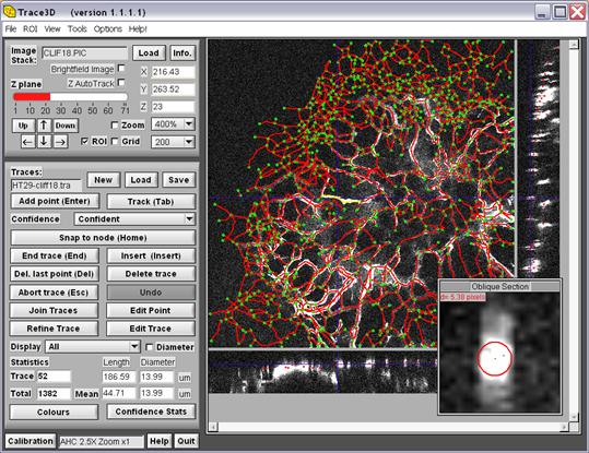
 The
image volume is displayed as 3 orthogonal sections, xy,
xz and yz (as shown in the
figure above). Usually, the volume has been acquired as a stack of xy images that provide views progressively deeper into the
sample. Deeper into the sample is represented by an increase in the z
direction. If a movie is the image source then increasing z will represent an
increase in time. The cross-hairs indicate where the xy,
xz and yz planes are with
respect to each other. The xz view shows the
cross-section through the volume at the position of the horizontal line in the xy view. The vertical line shows the position of the yz cross-section shown in the yz
view.
The
image volume is displayed as 3 orthogonal sections, xy,
xz and yz (as shown in the
figure above). Usually, the volume has been acquired as a stack of xy images that provide views progressively deeper into the
sample. Deeper into the sample is represented by an increase in the z
direction. If a movie is the image source then increasing z will represent an
increase in time. The cross-hairs indicate where the xy,
xz and yz planes are with
respect to each other. The xz view shows the
cross-section through the volume at the position of the horizontal line in the xy view. The vertical line shows the position of the yz cross-section shown in the yz
view.
Click on the zoom check-box to toggle the zoom between 100% and the
chosen value. The zoom can also be toggled with a mouse right-click, or
<ctrl-z>. The centre of the zoomed volume is the current xyz position on
zooming in. To change the zoom centre to a new position, toggle the zoom out
and then in again; the new zoomed view will re-centre to the current xyz
position.
To improve image visibility,
‘Pre-Processing’ allows the image contrast to be stretched or normalised.
1.2
Navigation
Use the mouse to Click-left on
the xy, xz or yz views to place the cross-hair within the 3D volume. The
z position can also be set using the ‘Up’ and ‘Down’ buttons (‘Page Up’
and ‘Page Down’ keys) or the red slider. The xy
position can also be set using the arrow buttons (duplicated on the
arrow keys). The current position is shown in the x, y, z
numeric boxes. You can enter numbers here to jump to a specific (x, y, z) coordinate.
1.3
Traces
‘Load’ allows a previously saved
file of traces to be loaded. ‘Save’ saves the traces currently in memory. The
‘*.tra’ files used are unique to this application but
are simple text files that can be viewed in many applications (e.g. Word).
An example file:
Trace3D_file Title
2
Number of traces
8
Number of points defining trace 1
128.0
257.875 9.0 0 3.34 x y z coordinate, confidence, radius point
1
127.125
256.75 9.0 0 3.54 .
125.875
255.875 10.0 0 2.98 .
124.375
255.75 11.0 0 3.05 .
123.5
256.875 10.0 1 3.12 .
123.25
257.625 9.0 1 3.22 .
123.375
258.125 9.0 1 3.21 .
124.25
258.25 9.0 1 3.19 x y z coordinate, confidence, radius point
8
4
Number of points defining trace 2
130.5
278.875 39.0 0 –1.0 x y z coordinate, confidence, radius point 1
134.5 281.0
39.0 0 –1.0 .
138.75
279.125 40.0 0 –1.0 .
140.875
273.875 45.0 0 –1.0 x y z coordinate, confidence, radius point 4
‘Export’
can be used to make a VRML 2.0, *.wrl, file. This
virtual reality script will produce a 3D world that can be explored using a
VRML viewer such as the Cortona plug-in client for
Internet Explorer from Parallel Graphics (www.parallelgraphics.com). These
files can also be imported into Imaris Surpass and
viewed overlaid onto 3D rendered views of the original data.
The
traces can be rendered as lines of single pixel width or as cylinders with a
diameter that represents the measured diameter.
1.4
Display
Traces will be drawn on the xy, xz and yz
views in the colour selected (red by default). Node points (green by default)
mark the trace start and end points. Traces that have be
made with different confidences will be shown in different colours which can be
chosen in the options. The ‘Display’ menu allows the viewing of no traces (‘None’);
traces, and parts of, that cross the current z plane (‘Plane by Plane’) and
‘All’ traces regardless of position in space. Additional display modes are used
to speed up display updates, these are “last 10”, “last5” and
“last only” which display just the last few traces as indicated by the
nomenclature. The “Backspace” key (←) toggles between the current display
setting and “None” for convenience.
1.5
Tracing
Position the cross-hairs at the
start position for the trace in 3D space. Press <Enter> or click ‘Add
Trace Point’. Position the cross-hairs at the next position along the vessel
and press <Enter> or click ‘Add Trace Point’ again. Repeat to the end of
the vessel. Vessels can also be drawn or traced directly by holding
<Ctrl> whilst dragging the cross-hairs through the xy
view.
In addition to this, if “always
measure diameters” is selected in the options menu, an automatic diameter
measurement will be made for each point added. This will be shown in a small
pop-up window. The window will display an oblique cross-section through the
data, perpendicular to the current trace direction and the measured diameter
will be shown in red. The centre of the object will also be detected and the
trace point will automatically move to this centre (this can be disabled in the
options). These measurements can be corrected manually at this stage by
left-clicking on the window at the correct object centre and then dragging the
mouse to show the correct diameter.
To end the current trace, click ‘End
Trace’ or press the <End> key. The last point changes into a node.
To start tracing from a node,
position the cross-hairs near to the node and click ‘Snap to Node’ or press the
<Home> key. The current position will snap on to the nearest node (N.B.
the nearest in 3D space is not necessarily the closest on the xy view). Now press <Enter> or click ‘Add Trace
Point’ to start a new trace.
The <Delete> key and the
‘Delete last node’ button will delete back along the current trace. <Esc>
and ‘Abort Trace’ delete the current trace. To delete whole traces the ‘Delete
last trace’ button can be used.
1.6
Z
AutoTrack
The Z AutoTrack
function aids tracing in 3D by automatically moving the cross-hairs through z
towards the brightest point. This occurs when to z AutoTrack tick-box is on and you navigate in xy by clicking on the xy view,
clicking the arrow buttons or pressing the arrow keys. The idea is that as the
user traces a vessel in the xy view the AutoTrack
function will automatically trace the vessel in the third (z) dimension.
However, care must be taken when tracing weak/dim vessels as the function will
always prefer strong/bright structures.
The
‘Z AutoTrack options’ allow you to tell the system whether you are tracing
bright or dark structures and to set the size of smoothing filters used.
1.7
Statistics
The number of traces (vessels)
currently in memory is reported together with their mean length and diameter in
calibrated units. The length of the current, selected, or last, trace is also
given.
2
Controls
2.1
Load,
Image
‘Load’ will allow a Biorad image stack (*.PIC) or a
movie (*.AVI) file to be imported. Select the file from the file select pop-up
which appears.
2.2
Info.
Displays text details about the image stack currently
loaded in a text window. For a Biorad image stack this will be the “header” and
“notes” information. For a movie the relevant “header” information will be
shown.
2.3
X,
Y and Z
These controls show the current position of the
navigation cross-hair cursor in the image volume. The position can be changed
by entering numbers into these boxes.
2.4
Brightfield
Image
Check this box if the image you are
using was acquired on a brightfield microscope. Leave it blank if it is an
image of fluorescence (including multi-photon microscopy). This lets the
software know whether we expect the structure to be traced to be dark
(brightfield) or light (fluorescence) and enables the Z auto track and
automated tracing functions.
2.5
Z
AutoTrack
Turn off or on the z auto tracking. The Z AutoTrack function aids tracing in 3D by automatically moving
the cross-hairs through z towards the brightest point. This occurs when
to z AutoTrack tick-box is on and you navigate in xy
by clicking on the xy view, clicking the arrow
buttons or pressing the arrow keys. The idea is that as the user traces a
vessel in the xy view the AutoTrack function will
automatically trace the vessel in the third (z) dimension.
However, care must be taken when tracing weak/dim vessels as the function will
always prefer strong/bright structures.
2.6
Z
plane, Up and Down
You can quickly change the current z plane displayed
by using this slider. The ‘Up’ and ‘Down’ controls also step through the image
volume, displaying different z planes (The Page Up and Page Down keys on the
keyboard also operate these controls).
2.7
Arrow
Keys
You can move around the xy
image in precise steps using these controls which are also operated by the
arrow keys on the keyboard. If a trace has been selected by a double-left-click
the arrow keys allow you to move along the trace point by point. Left or down
moves toward the start of the trace, right or up move toward the end.
2.8
Zoom
Click on this zoom check-box to toggle the zoom
between 100% and the chosen value. The zoom can also be toggled with a mouse right-click, or
<ctrl-z>. The centre of the zoomed volume is the current xyz
position on zooming in. To change the zoom centre to a new position, toggle the
zoom out and then in again; the new zoomed view will re-centre to the current
xyz position.
2.9
ROI
This option
displays the Region Of Interest (ROI) on the image. The ROI can also be toggled with
<ctrl-r>.
2.10 Grid
This option
puts a grid on the image to make it easier to progressively trace a large
image. The size of the grid can be set with the adjacent pull-down menu. The grid can also be toggled
with <ctrl-g>.
2.11 Traces: New
This control clears all the traces from memory to
start a new set of traces.
2.12 Traces: Load
This load control can be used to load into memory a
previously saved set of traces.
2.13 Traces: Save
This control will save the set of traces currently in
memory. The first time this is used you will be prompted for a file name (As
with the ‘Save Traces As’ menu command). Subsequently the same file name will
be used.
2.14 Add Point (Enter)
Inserts a trace point at the cursor position. If no traces are started this
starts a new trace. If a trace has been started this continues it. TIP: You can also make traces by
just holding <Ctrl> whilst moving the mouse over the xy
image.
2.15 Track (Tab)
Starts automatic tracking of
position and diameter of the object being currently traced. The trace must already have at least two good points, which are usually
manually traced. Automatic tracking will stop when a good object of suitable
radius can be found. It will track over node points and it is suggested that
node points are inserted afterwards. Tracking can be forced to stop by clicking
the red “Stop” button.
The
automatic tracking can be adversely affected by noisy data. Please experiment
and check the results with your data.
2.16 Confidence
Sets the
confidence for subsequent points added to a trace.
2.17 Snap to node (Home)
This
control will move the navigation cursor to the nearest node point.
2.18 End trace (End)
End the
current trace and mark the end with a node.
2.19 Insert (Insert)
This is available when a trace has been selected by a
double-left-click on the trace. This control inserts a node or extra points
near the selected point. A pop-up panel asks whether you want to insert a node
into the current trace (i.e. split the trace into two) or insert a point in
between the current point and its neighbour (either before or after it in the
trace). An inserted point will appear half way along the line linking the two
points and after insertion can be moved to by pressing the left or right arrow
key.
2.20 Del. Del
Deletes points from the end of
current trace. If the last trace has been ended
with a node, this control will delete the node to allow tracing to continue.
Repeated action of the control will delete the trace point by point. If a trace
has been selected by a double-left-click on it, this control will delete either
the node or point from the end nearest the selected point.
2.21 Delete Trace
If a trace
has been selected by a double-left-click on it, this control will delete it.
2.22 Abort Trace (Esc)
This will
delete a trace that has been started but not ended. If a trace has been
selected by a double-left-click on it, this control will de-select it.
2.23 Undo
A single
undo step is available for some actions. The control will become bold when
available and dimmed when the last action cannot be undone.
2.24 Join Traces
Allows two traces to be joined at their end points. Select a trace by a
double-left-click on it, then press this control. The
computer will find the nearest end of the trace selected, and then find the
nearest end of another trace and propose that they be joined. The proposed
joint will be shown as a new trace in the colour of a selected trace (default
yellow), click on “Yes” to make this joint, “No” to find the next nearest end to
join to, or choose “Cancel”. N.B. if you are joining two traces which already
end at the same point, the proposed joint will not show up. If three traces end
at this point, or very close together, you may need to delete one or more
points back on some traces in order to see the proposed joints. If a mistake is
made then the joined trace can be split again with the “insert” function.
2.25 Edit Point
This is
available when a trace has been selected by a double-left-click on the trace
and displays a window with the parameters of the selected point (x, y, z,
radius and confidence) which can be edited manually.
2.26 Refine Trace
This is
available when a trace has been selected by a double-left-click on the trace
and re-measures the diameter and centre position along the trace. Used
repeatedly this often refines the position of the trace on the structure. It
uses the same options as tracking including the watch tracking option which can
be used to view the diameter measured in a pop-up window.
2.27 Edit Trace
This is
available when a trace has been selected by a double-left-click on the trace
and displays a window with the parameters of the selected trace (radius and
confidence) which can be edited manually. These actions will set the radius or
confidence for the whole trace (every point).
2.28
Display
Traces
will be drawn on the xy, xz
and yz views in the colour selected (red by default).
Node points (green by default) mark the trace start and end points. Traces that
have be made with different confidences will be shown
in different colours which can be chosen in the options. The ‘Display’ menu
allows the viewing of no traces (‘None’); traces, and parts of, that cross the
current z plane (‘Plane by Plane’) and ‘All’ traces regardless of position in
space. Additional display modes are used to speed up display updates,
these are “last 10”, “last5” and “last only”, which display just the last few
traces as indicated by the nomenclature. The “Backspace” key (←) toggles
between the current display setting and “None” for convenience. TIP: If you have a mouse with
additional buttons you may be able to assign the backspace key to one of those.
Diameter
Check
this box to display each trace with a thick line that represents the diameter
of the trace. This can be used to quickly see which traces have a diameter
measurement and whether the measurements are reasonable. TIP: <Ctrl-d> is the
shortcut for the command.
2.29 Statistics
The number
of traces (vessels) currently in memory is reported together with their mean
length and diameter in calibrated units. The length of the 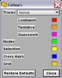 current, selected, or last, trace is
also given.
current, selected, or last, trace is
also given.
2.30 Colours
Opens a pop-up panel to allow the trace display colours to be changed.
2.31 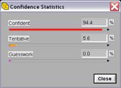 Confidence Stats
Displays a window showing the proportion of traces that have been marked
with different confidence levels.
2.32 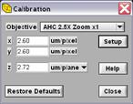 Calibration
Can be
used to assign real distances to x, y, and z. These numbers are used to
calculate trace/vessel lengths and can be used to export VRML scripts in real
coordinates. Use the ‘Setup’ command to change the preset settings for
different objectives. The selected objective is shown in the adjacent text box.
2.33 Help
‘Help’ shows this document.
2.34 Quit
‘Quit’ quits the application!
3
Menus
3.1
File
3.1.1
Load
Image Stack
Echos the
‘Load’ control and will allow a Biorad image stack (*.PIC) or a movie (*.AVI)
file to be imported. Select the file from the file select pop-up which appears.
This
control clears all the traces from memory to start a new set of traces.
3.1.2
New
Traces
This
control clears all the traces from memory to start a new set of traces.
3.1.3
Load
Traces
This load control can be used to load into memory a
previously saved set of traces.
3.1.4
Save
Traces
This control will save the set of traces currently in
memory. The first time this is used you will be prompted for a file name (As
with the ‘Save Traces As’ menu command). Subsequently the same file name will
be used.
3.1.5
Save
Traces As
This control will save the set of traces currently in
memory to a filename you can define. The new filename will then be used by the
save commands.
3.1.6
Export
Traces
 ‘Export’ can be used to make a VRML 2.0, *.wrl, file. This virtual reality script will produce a 3D
world that can be explored using a VRML viewer such as the Cortona
plug-in client for Internet Explorer from Parallel Graphics (www.parallelgraphics.com). These
files can also be imported into Imaris Surpass and
viewed overlaid onto 3D rendered views of the original data.
‘Export’ can be used to make a VRML 2.0, *.wrl, file. This virtual reality script will produce a 3D
world that can be explored using a VRML viewer such as the Cortona
plug-in client for Internet Explorer from Parallel Graphics (www.parallelgraphics.com). These
files can also be imported into Imaris Surpass and
viewed overlaid onto 3D rendered views of the original data.
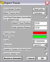
On the
‘Export Traces’ panel you can specify whether the virtual world uses the real
units from the ‘calibration’ panel or is simply in uses pixel dimensions. The traces can be rendered as lines of single pixel width or as
cylinders with a diameter that represents the measured diameter. If cylinder
rendering is asked for but the diameter for some traces has not been measured
then the default radii are used and can be specified here. Trace and Node
colours can be specified. The scale of the virtual world can be changed to suit
you viewer. ‘Export as’ sets the export language.
The virtual rendered traces can have their origin at
the data (0,0) or at their own centre which is
achieved by checking the ‘Create in Centre of Virtual World’ box. If you want
to view the world now then check the ‘Launch viewer now’ box.
3.1.7
Quit
Quits the application.
3.2
ROI
A region of interest (ROI) can be
defined and will appear on the xy image view if the
ROI box on the front panel is checked. This allows you to select traces that
are wholly contained within the ROI and save them to a new trace file (*.tra).
3.2.1
Define
Region Of Interest (ROI)
Opens a new
panel that allows you to define, change, load or save the ROI. The ROI can be
changed using the shape tool that appears on the main image view.
3.2.1.1
Tool
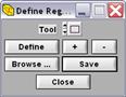 This chooses the shape that can be
added or subtracted to the ROI.
This chooses the shape that can be
added or subtracted to the ROI.
3.2.1.2
Define
Defines the ROI as the current shape. The previous ROI will be lost.
3.2.1.3
+
Adds the current shape to the ROI.
3.2.1.4
–
Subtracts the current shape from the ROI.
3.2.1.5
Browse
Lets you
browse for and load any bmp image as a ROI. All zero pixels will be outside the
ROI, all non-zero pixels will be inside.
3.2.1.6
Save
Lets you
save the current ROI to a bmp file.
3.2.1.7
Close
Use this
button to close the Define ROI panel before continuing.
3.2.2
ROI
Information
Changes the ROI to an oval shape.
3.2.3
Save
Traces in ROI
Changes the
ROI to an oriented quadrant for selecting a quadrant of a
oval object.
3.3
View
3.3.1
File
Information
Displays text details about the image stack currently
loaded in a text window. For a Biorad image stack this will be the “header” and
“notes” information. For a movie the relevant “header” information will be
shown.
3.3.2
Confidence
Stats
Displays a window showing the proportion of traces that have been marked
with different confidence levels.
3.4
Tools
3.4.1
Pre-Processing
This control opens a pop-up window that allows you to control how the
images are displayed.
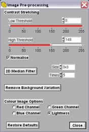
3.4.1.1
Contrast
Stretching
The low and high thresholds allow you to increase the
image contrast; any data below the low threshold will be displayed black and
any data above the high threshold will be displayed white. The images can also
be normalised by checking the box, this shows the lowest values in the image as
black and the highest as white and is performed separately for the xy, xz and yz
images.
3.4.1.2
2D
Median Filter
A 2D median filter can be applied to all the xy images in the stack. Please select a kernel size (amount
of smoothing per pass) and the number of times to apply (number of passes) and
click ‘2D median Filter’.
3.4.1.3
Remove
Background Variation
This experimental option can be used to remove broad
variations in the background illumination or surrounding tissue.
N.B.
There is no undo function for the last two operations. If you mess up, the best
thing to do is reload the image.
3.4.1.4
Colour
Image Options
If a colour image has been loaded then you can choose
which colour channel to perform the tracing on. Select each one in term and
choose the one with the best contrast.
3.4.2
Refine
Trace
See here.
3.4.3
Refine
All Traces
The Refine
All Traces menu option was added for testing vessel diameter measurement; setup
start traces on the known centre of the vessels with radius -1 or guess value,
then select refine all to measure the diameter at each point (make sure Kalman filering is OFF). Measure
all will do the same but will not move the centre position.
3.4.4
Measure
Diameter
This is
available when a trace has been selected by a double-left-click on the trace
and measures the diameter at the selected point. This is displayed in a pop-up
window. This measurement can be corrected by clicking and dragging an object
radius on the window.
3.4.5
Measure
diameters of all traces
Allows the measurement of diameters along traces already made. For instance, traces from a
previous version of this software where diameter measurement was not possible.
You are asked whether you want to measure diameters for all vessels or just
those without a measurement yet (radius = -1) before proceeding. The measurement can be forced to stop by clicking the red “Stop”
button.
3.4.6
Automatic
2D Tracing
Open a new
panel to setup and start the automatic tracing algorithm. This currently only
work for 2D images and is still under development. Please try it!
3.4.7
Trace
Statistics
Opens a new
panel used to report statistics about the traces. See.
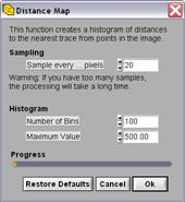
3.4.8
Euclidean
Distance Map
This
creates a histogram of distances to the nearest trace from all, or a sample of,
points in the image. You specify in “Sampling” how often to take a point to
measure the distance for. Setting this to 1 samples
every point. The sampling applies in x, y and z. In cases where the image
dimension is less than the sampling distance, you will get one sample in that
dimension (e.g. if there are only 10 z-planes in the image but sampling is set
at 20). You can define how many bins and what the maximum value of the
histogram should be.
3.4.9
Fractal
Dimension
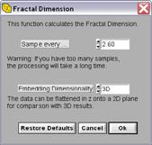 This calculates the fractal
dimension of the traces using the ‘Box Counting’ method via the ‘fd3’ algorithm
(see here). The traces are first converted into
a list of points and the sampling rate
This calculates the fractal
dimension of the traces using the ‘Box Counting’ method via the ‘fd3’ algorithm
(see here). The traces are first converted into
a list of points and the sampling rate
3.5
Options
3.5.1
Z
Auto-Track
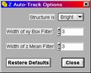 Displays the options panel for Z Auto-Track (see here). Define whether the structure you
want to snap onto is bright or dark with respect to the background with the
‘Structure is’ control. Data about the cursor point is filtered in xy and in z to make the auto-tracking more robust. Two controls
allow you to specify the degree of filtering by setting the width of these
filters. Higher numbers mean more filtering which may be necessary for very
noisy data.
Displays the options panel for Z Auto-Track (see here). Define whether the structure you
want to snap onto is bright or dark with respect to the background with the
‘Structure is’ control. Data about the cursor point is filtered in xy and in z to make the auto-tracking more robust. Two controls
allow you to specify the degree of filtering by setting the width of these
filters. Higher numbers mean more filtering which may be necessary for very
noisy data.
3.5.2
Colours
See here.
3.5.3
Calibration
See here.
3.5.4
Object
Tracking
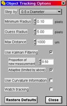 Displays the
options panel for object tracking. The tracker steps along the object
determining centre position and radius at each step. The step size can be set
with the ‘Step by’ control, and can be a proportion of the measured diameter or
simply continue with the same separation of the last two points (‘Last Point
Separation’).
Displays the
options panel for object tracking. The tracker steps along the object
determining centre position and radius at each step. The step size can be set
with the ‘Step by’ control, and can be a proportion of the measured diameter or
simply continue with the same separation of the last two points (‘Last Point
Separation’).
The ‘Minimum Radius’ control sets the absolute minimum radius allowed
for any object.
If a radius of less than this value is measured then tracking of that object
will stop. The ‘Guess Radius’ initialises the radius measurement for new traces
with no previous radius measurements. This value need only be approximate. The
Max Distance control sets a limit on how far the tracker can go.
A Kalman filter can be used to add robustness to the
tracking. The proportions of predicted and measured values for position and
diameter can by fixed on this panel. Alternatively the filter can be allowed to
adapt to how well it thinks the diameter measurement has been made in
determining the next point. The adapted value will never go above the
proportion value given.
In theory,
the use of curvature information should make the prediction of the next point
better. This does not seem to be the case in practice. The “Use Curvature
Information” box is best left unchecked (on the other hand, there may be a bug
in the code!).
You can
monitor the progress of the tracking and diameter measurement by checking the
“Watch tracking” box.
3.5.5
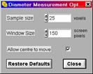 Diameter Cross-section
Sets the Diameter measurement and cross-section display options. The ‘Sample size’ sets the number
of voxels that will be used to make the oblique
cross-section. A value of 25 means that data will be taken
from a 25 by 25 square around the object centre. The ‘Window Size’ is
the size of the pop-up window in pixels, a value of 150 means that the 25 by 25
cross-section will be magnified to fill 150 by 150 for display.
‘Allow
centre to move’ specifies whether the centre of the object is allowed to move
when measuring the diameter via the ‘Measure Diameter’ control or when manually
tracing. This does not effect the automatic object
tracing.
3.5.6
Always
Measure Diameter
If this is
checked then the diameter will be measured during manual tracing.
3.5.7
Cross
Hairs
If this is
checked the full cross
hairs will be shown across the image to indicate the current
cursor position.
3.6
Help!
Shows this help document.
4
Trace Statistics
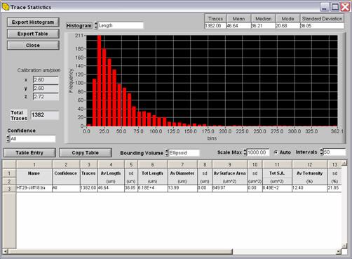
4.1
Histogram
Choose the
data to be analysed from Length, Diameter, Volume, Surface Area or Tortuosity. The histogram for those data will be plotted
and statistics placed in the table top-left of the panel.
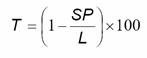
The
measurement of percentage tortuosity (T) was
equivalent to that of Norrby (Norrby,
K., Microvascular Research 55: pp 43-53, 1998) and is based on the distance between branching
points along the vasculature (L) and in a straight line (SP):
4.2
Scale
Max
Sets the
upper scale limit for the histogram unless the Auto button is checked in which
case the scale is automatically calculated.
4.3
Intervals
Sets the number of histogram bins or bars.
4.4
Table
Entry
Calculates
several statistics on the data histograms and places them in the table at the
bottom.
4.1
Copy
Table
Copies the table to the clipboard so that it can be pasted into another
application, such as Microsoft Excel.
4.2
Bounding
Volume / Area
Defines the
shape used to estimate the volume or area bounding the traces. See the 2D
examples below. The cuboid contains all the traces.
The ellipsoid is the largest that can fit in that cuboid.
Remember
that this bounding volume is just an estimate and does not take account of the
trace diameters. Strange results for the fill % can be gained if the traces are
wider than the image!
4.3
Export
Histogram
Lets you
save the histogram data in a text file for import into Microsoft Excel, for
example.
4.4
Export
Table
Lets you
export the entire lower table to a text file.
4.5
Close
Closes the trace statistics panel.
5
Synopsis of FD3
FD3 is a
program that estimates fractal dimension.
It was
written by John Sarraille and Peter DiFalco, using ideas from "A FAST ALGORITHM TO
DETERMINE FRACTAL DIMENSION BY BOX
COUNTING",
by Liebovitch and Toth,
Physics Letters A, 141, 386-390 (1989).
FD3 inputs
an ascii list of points,
basically one point per line, and outputs box counts at various scales, plus
estimates of capacity, information, and correlation dimension.
There are
"two-point" estimates of dimension for each scale shift (division of
cell size by two), plus overall estimates based on fitting a least-squares line
to a log-log plot of cell count versus cell size.
FD3 is
quite accurate (typically well within 5% when tested on reasonably-sized
samples of fractals whose dimension are known exactly)
It is quite
fast -- O(NlogN) where N is
the number of data lines (points) input.
In theory,
it will handle any embedding dimension – points with one coordinate each, two
coordinates each, three, four,
... whatever. However,
the number of points needed for usable results increases geometrically with the
dimension of the set.
For more
information on how to use FD3, see the files INDEX, README.2, and REPORT.INF
/* BEGIN
NOTICE
Copyright
(c) 1992 by John Sarraille and Peter DiFalco (john@ishi.csustan.edu)
Permission
to use, copy, modify, and distribute this software and its documentation for
any purpose and without fee is hereby granted, provided that the above
copyright notice appear in all copies and that both that copyright notice and
this permission notice appear in supporting documentation.
The
algorithm used in this program was inspired by the paper entitled "A Fast
Algorithm To Determine Fractal Dimensions By Box
Counting", which was written by Liebovitch and Toth, and which appeared in the journal "Physics
Letters A", volume 141, pp 386-390, (1989).
This
program is not warranteed: use at your own risk.
END NOTICE
*/