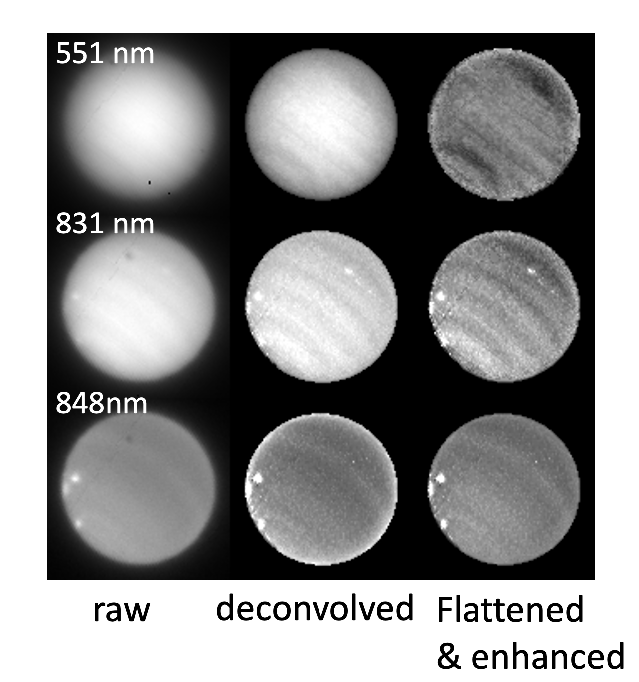
Spatial deconvolution

Ground-based telescopic obseervations of the planets are limited in their spatial resolution by the turbulence of the Earth's atmosphere. This effect, known as 'seeing', is what makes the stars twinckle and through an amateur telescope can be seen as 'shimmering' or 'wobbling' of the image. The world's best telescopes are located in regions where the overlying air is especially stable, such as in Hawai'i, or in the Atacama Desert of Chile, but even in the best conditions, the best spatial resolution at visible wavelengths is usually limited to roughly 0.5 arcsec (or 0.5"). Given that the maximum size of Neptune's disc is only 2.4" this represents a considerable blurring. More usually the 'seeing' is of the order of 1 arcsec, and so even large planets, such as Jupiter, which has a diameter more like 40", the blurring is significant.

To counteract this effect, large telescopes now regularly use 'adaptive' optics to improve the image quality. This system uses a nearby star in the image field, or if this is not available a synthetic star created by shining a laser in the same direction as the object and stimulating flourescence of a layer of sodium atoms in Earth's atmosphere at an altitude of roughly 30 km above the surface. The wavefront from this star, which if there is no trubulence, should be planar, is continuously monitored by the adaptive optics system which controls in real time a secondary, deformable mirror in the optical chain that ensures the wavefront at the detector from the star is planar. This removes the 'seeing' blurring from the star, but also anything else in the field of view, and enables such systems to improve the spatial resolution to something morew like 0.1 or 0.2", although the performance gets worse a shorter, bluer wavelengths.

In our recent Neptune Dark Spot paper, we analysed observations of Neptune made in 2019 with the Multi Unit Spectroscopic Explorer (MUSE) instrument on the Very Large Telescope (VLT) in Chile. We hoped that the spatial resolution of VLT/MUSE would be sufficient to image a new dark spot, NDS-2018, that was present in our data. However, while the spatial performance was good at longer wavelengths, it was not quite sufficient at blue wavelengths to discriminate the spot. As a result we had to develop new method of 'deconvolving' the observations. This is discussed in detail in our dark spot paper, but here we have reproduced the main points for ease of reference, below.

Our deconvolution package, modified-clean, was developed primarily by one of my post-docs, Jack Dobinson, under a grant from the UK's Science and Technology Facilities Council (STFC). Jack Dobinson is now supported to further develop this technique via a grant from the Leverhulme Trust.

The technique we have developed, which we call modified-clean, is modified version of the clean} algorithm of Hobgom (1974). Instead of single point subtractions, pixels above some selection threshold, t_s, are convolved with the instrumental PSF and a fraction of the result, the loop-gain g_loop, subtracted from the "dirty map" at each iteration. For this method to work we need to have an observation of standard star, which was recorded at neartly the same time, with the same airmass and cloud conditions. In our model t_s is determined dynamically by choosing an initial threshold, t_i, from successive applications of 'Otsu' thresholding (Otsu, IEEE T. Syst. Man Cyb. 9, 62–66, 1979), and applying a user-supplied factor, t_factor (which we typicaslly set to 0.3), to the interval between t_i and the data maximum such that \[ t_\textrm{s} = (\textrm{data maximum}) \times t_\textrm{factor} + (1 - t_\textrm{factor}) \times t_\textrm{i}. \] Otsu thresholding is a method of separating an image into two different classes of pixels (generally the background and foreground, or dark and bright) by choosing the threshold that minimises the variance of the two classes. modified-clean works best when small bright features are deconvolved before larger features, therefore successive rounds of Otsu thresholding were applied to the bright classes until the newest bright class contained a single pixel, or a maximum of 10 iterations. The single threshold that best selected small bright regions compared to the other candidate thresholds was chosen as t_i via an "exclusivity", e_x, measure.

When choosing t_i, for each Otsu threshold, t_otsu, considered, e_x is calculated using the fraction of selected pixels, f_pix = N_bright/N, and the fraction of rejected range, f_range = (t_otsu - min)/(max - min), where N is the number of pixels in the range of values, t_otsu is the computed Otsu threshold, N_bright is the number of pixels above t_otsu, and min and max are the minimum and maximum values of the pixels in the range of values being considered. Combining these together gives the exclusivity as \[ e_x = (f_\textrm{range} - f_\textrm{pix})/(f_\textrm{range} + f_\textrm{pix}). \] Of the candidate values of t_otsu considered, the one with the highest e_x is chosen to be the initial threshold t_i, from which t_s is computed.

Once the deconvolution is complete and the component delta-functions (modified-clean-components) are found, we do not re-convolve the final modified-clean-components with a "clean beam" as is standard practice. This is because one of the main goals of this deconvolution is to remove the "halo glow" effect of the adaptive optics, which significantly impacts limb-darkening Minnaert parameter estimations made from the original data.

Before deconvolution, instrumental artefacts, missing data, and features smaller than the PSF can be identified using an algorithm based on singular spectrum analysis (SSA) and interpolated over. This reduces the number of iterations required and ameliorates one of the main problems with the family of clean algorithms, their propensity to form speckles and ridges even with modifications.