Graph Networks of Protein Folding With Contact Maps Leads to Markov State Models

Introduction

Protein folding is still a difficult problem. Although AlphaFold made great strides in advancing static structure prediction, the dynamic process that transports a protein from random coil to equilibrium structure is difficult to model. Go based Ising-like energy models such as the WSME model were among the first successful mathematical models of protein folding as a kinetic process. The approach is as follows: given a native-like folded conformation, we can assign residues with any possible alternative conformation as either native-like or not. One way to define this is to consider the residue’s formation of native-like contacts ($C_\alpha - C_\alpha$ distance $<8\dot{A}$). In folding this could be the difference between a random coil unfolded state where a given residue makes few native-like contacting pairs with spatially proximal residues, versus the folded state where that residue may exist in an alpha helix.

The Ising-like approach is to simply formulate the protein with a binary state for each residue, taking 1 if that residue is in the native-like conformation and 0 otherwise. The WSME model itself is specifically formulated so that the associated Ising-like hamiltonian is combined with an entropic parameter for each residue resulting in a canonical Free energy functional. The model is therefore kinetically meaningful and approximates a protein’s folding free energy landscape. For a more detailed description of the WSME model see Ooka, Liu, Arai. 2022.

What I’m hoping to illustrate with reference to the WSME model is that modelling protein folding as a dynamical process of state transitions is well established. What’s cool is that such state-based formulations lend themselves well to graph networks, which, alongside being great visualisation tools, also allow for a number of powerful mathematical analyses. So, what can we learn from graph network representations of protein folding?

Throughout this blog I will specifically consider molecular dynamics (MD) simulations of protein folding, namely that of the 10 residue artificial fast folder Chignolin. Naturally this means we are modelling numerical physics-based approximations of protein folding rather than experimental data such as SAXS and HX. The reason for this is because MD trajectories are trivial to interpret and prepare, and for a number of well described fast folding proteins, are accessible and reproducible.

Contents

• Building a Graph - Methods
• Scrutinising the Shortest Path
• The Physics of Folding
• Identifying the Transition State Ensemble
• Take Homes

Methods

Like the WSME model I’m going to rely on residue contacts to define a protein’s state in folding. Specifically, we will consider every unique contact map ($N_{\text{res}} \times N_{\text{res}}$ boolean matrix) of a protein as a possible state that the protein can take during folding - these will be the nodes of our graph. Where edges represent relationships between states we can define them as follows: Given an MD trajectory of protein folding we may want to draw edges between nodes if the respective two contact maps are at any point adjacent in sequence in the trajectory - in other words, if node $i$ is the contact map of frame $t$ in the trajectory, we draw an edge from $i$ to $j$ if the contact map of either frames $t-1$ or $t+1$ belongs to node $j$. The below image is one such graph network for the artificial fast folding protein Chignolin (10 residues) using the trajectory data from Majewski et al. 2022 who repeated the original simulations from Kresten Lindorff-Larsen et al. How Fast-Folding Proteins Fold: 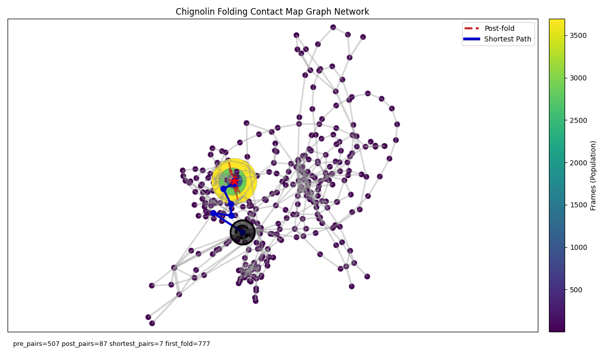Figure 1: Graph where nodes represent unique contact maps and edges connect temporally adjacent nodes. Node size corresponds to its respective contact map’s count in the folding trajectory. Nodes are coloured by the index in the trajectory of the first occurrence of their respective contact map. The outlined black node indicates the starting frame node (the unfolded conformation). Blue edge colouring highlights the shortest path to the yellow folded node whilst red edge highlighting indicates post-folded state transitions.

Immediately we can spot something interesting. The largest node (yellow) represents the most commonly visited unique contact map in the trajectory which, given this is a folding simulation, we might assume is the folded conformation. This state is surrounded by a number of nodes that are visited only after the folded state is reached. Indeed by colouring edges appearing after reaching that state with red, we can see that the protein, upon reaching its folded state, seems to bounce around exclusively within this small basin. On the other hand we see the comparatively large space explored by the protein before reaching this ensemble, depicting the protein’s search over the folding landscape.

However, as this graph is constructed purely by temporal edge information there is no physical meaning to its coordinate system - if nodes are close together this is just a product of the graph building algorithm. Let’s keep our temporal edges visible but overlay them on a graph who’s real edges are defined by adjacency in the space of all contact maps. In other words, nodes $i$ and $j$ are connected if they differ by exactly one contact. This forms an $N_{\text{residues}}^2$ dimensional discrete hypercube manifold which we can project to 2D coordinates by embedding with UMAP to get the following: 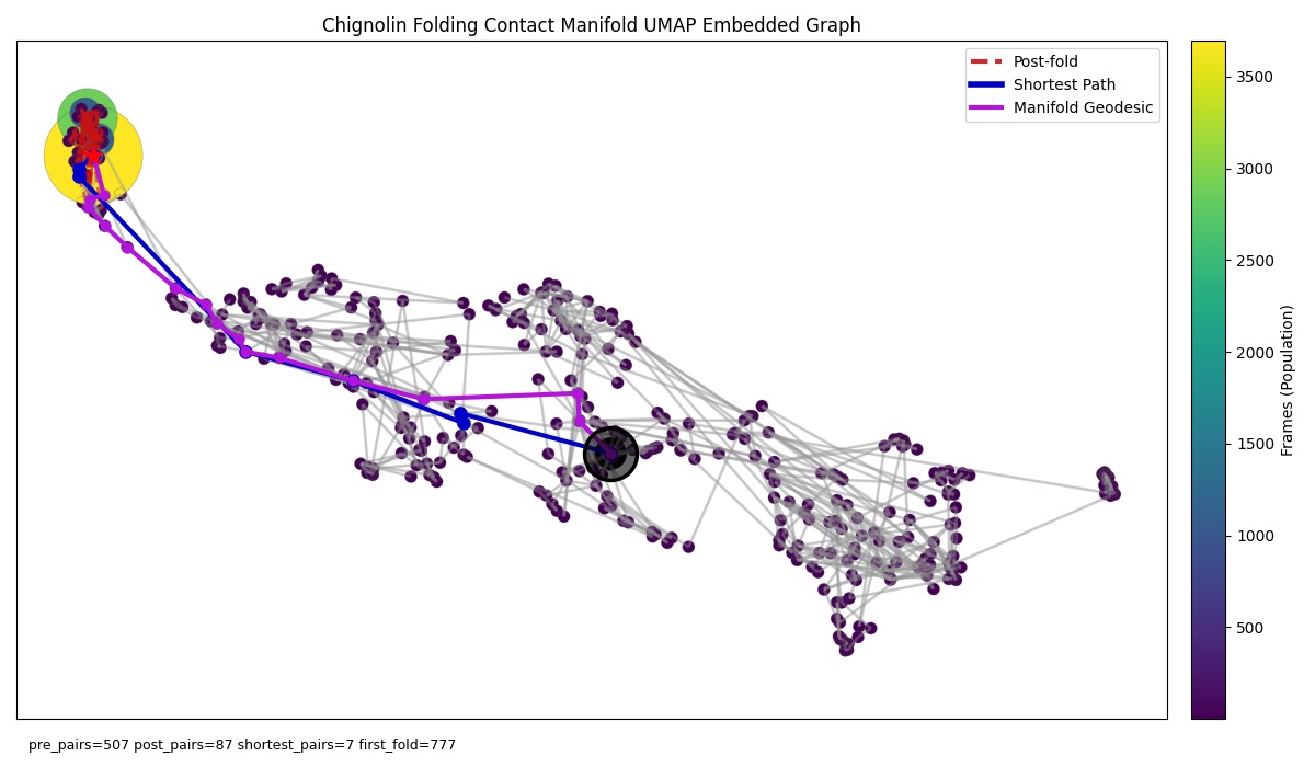Figure 2: Unlike the previous graph node connectivity is defined by adjacency on the discrete contact map configuration space manifold and projected down to a 2D representation to approximate differences in structure between nodes. Violet edge colouring represents the shortest path adhering strictly to the underlying manifold edges (manifold geodesic)

Again we observe how the folding process as a somewhat inefficient search over the contact map space bottlenecked by a number of key nodes. This raises the question of why all of the space to the right of the starting state is explored before reaching the first transition considering that the progression to the folded state is clearly left-directional - although I must emphasise that geometry is still not equivalent to reaction coordinate in this graph (see later). Is this due to inefficiencies in nature’s folding machine, inaccuracies in the MD approximate physics, or perhaps an apt visualisation of the initial random search theory of protein folding posited by Dill & Chan 1997.

One thing we can reveal from taking the intersection of manifold and temporal edges (edges that only appear in both sets) is that the unfolded state is a non-continuous process disconnected from the folded state along the discrete manifold space - this isn’t anything surprising it just means this flip is likely hidden under temporal transitions consisting of multiple contact flips. Specifically the 3rd edge on the manifold geodesic (ASP2, THR5) is never observed in the set of temporal edges, the protein navigates around it rather than making the direct link. (ASP2, THR5) is also not a native contact.

Although we constructed our graph in the contact map manifold space by defining node connectivity by a Hamming distance of 1, the coordinate system the graph is projected onto is still not super meaningful as it is now a product of the graph construction engine applied to UMAP embeddings. Instead we can take this a step further and use multidimensional scaling (MDS) which attempts to place nodes in 2D so that their physical distance is proportional to the Hamming distance between them (number of different unique contact pair flips). Here’s what that looks like: 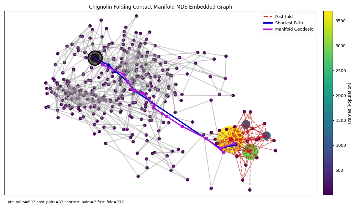Figure 3: Now node positions are explicitly defined by the MDS embedding. For this graph I actually used 10 components for the MDS embedding and simply plotted the first 2 dimensions for each node. So distances in this graph are physically true to the first 2 dimensions which should capture most of the variances but may lead to different clustering behaviour.

It’s a bit uglier but this appears to better depict the funnel like nature of protein folding. In both of these manifold graph representations the shortest paths (blue and violet) are still the same sequence of nodes but now our MDS representation depicts the actual distance from unfolded to folded in contact space.

Clearly Chignolin does not take either shortest path, why? It’s likely that some energetically favourable conformation must be reached before the large jump into the folded conformation can be achieved. Are these graphs just pretty or could they help us explore how to identify these transition states and ways to engineer proteins to more efficiently reach them without all the random search. Perhaps we can formalise these sentiments into a quantitative framework by drawing on the properties of these graphs.

Scrutinising the Shortest Path

The violet path represents the shortest path traversing only real contact map space edges, the manifold geodesic, but its construction requires bridging manifold nodes with edges not necessarily seen in the real trajectory. Let’s consider the blue shortest path from the previous plots, notice the particularly long edge jumping to the folded state, this is a temporal edge, not a real edge representing a contact flip on the manifold. Given the proximity and parallel nature of the manifold geodesic alongside this long edge we can assume the long edge is a cooperative event including the 5 single manifold edge flips of the manifold geodesic over a single 200ps snapshot.

Both are useful - the manifold geodesic represents the mechanistic pathway and the temporal edges the kinetics, together we gain useful insights. The relative speed of this simultaneous contact flipping implies a lower energistic barrier from their cooperation compared to temporal events traversing a single manifold edge. Let’s quantify this: 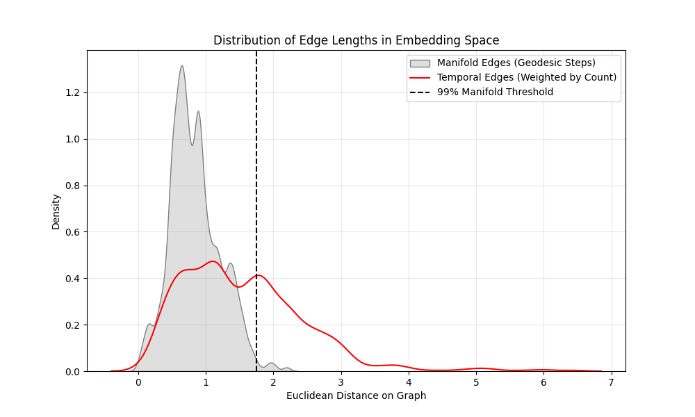Figure 4: Histograms of edge lengths for the manifold edges (grey area) and temporal edges (red outline).

Half of the temporal edges have a euclidean distance greater than 99% of the manifold edges on the MDS embedded graph. The conclusion I’m taking from this is that half of the temporal edges represent cooperative contact flip events. I leave it to the next blog to use this interesting property for estimating individual contact flip energies which would support models such as the WSME who’s $\epsilon_{ij}$ value is a simple heuristic.

The Physics of Folding

Previously we established shortest paths in the contact manifold space graph to be the most efficient paths from unfolded to folded with the minimal number of contact pair changes. Of course, in reality contact flips vary in energetic cost which we noted with the relationship between temporal edge length, time, and contact flip count. This is ultimately why the protein takes the long sporadic path we see in the trajectory. Let’s try to capture some idea of energetic cost in our graph edges by weighting them.

Imagine we have a weighted graph $G = (V,E,W)$ with nodes $V = \{v_1,...,v_N\}$, each representing a unique state (contact map), and edges $E = \{e_{ij}\}_1^j \quad \forall i,j \quad e \in [0,1]$ with weights $W$. We could take a thermodynamic approach to weighting edges taking inspiration from the WSME model which defines a free energy functional of a state $F(v_i)$ by its contacts:

$$ F(v_i) = \sum_{a,b} \epsilon_{ab}\Delta_{ab}(v_i) - T\Delta S(v_i), \quad a,b \in \{1,...,N_{\text{res}}\} $$

Where $S$ is the configurational entropy of the state, $T$ is temperature, and $\Delta_{ab}$ is a binary variable that is 1 if the residue pair $a,b$ is in contact. However, this requires us to set a value for the contact energy $\epsilon$ and a formulation for entropic cost.

Instead let’s view things from a thermodynamic perspective more typical of MD analysis. The simplest approach is with the classic free energy functional $F$ via Boltzmann Inversion from statistical mechanics which characterises transitions’ energetic cost:

$$ F_i^{\text{pseudo}} = - k_B T \operatorname{ln} \frac{M_i}{\sum_i^{N_{\text{nodes}}} M} $$

Where $k_B$ is the Boltzmann constant and $T=300K$ the temperature, and $M_i$ the state count at node $i$. We can approximate the population sizes of each state from their node sizes given that we have a sufficiently long enough simulation (given the ergodic hypothesis of MD). We can simply weight edges by the change in $F^{\text{pseudo}}$:

$$ W_{ij}^{\text{thermodynamic}} = \operatorname{max}\big(0,\;F^{\text{pseudo}}_j - F^{\text{pseudo}}_i\big) $$

This is a Metropolis acceptance essentially that assigns positive weight to uphill energistics and 0 to anything downhill making it instantaneous, giving us a formulation with a thermodynamic perspective which energy increases. The weakness to this approach is that it assumes ergodicity of the simulation (it has run long enough to reach equilibrium), e.g. the most populated state is assumed to be the most stable and therefore folded which was our original assumption.

On the other hand a Markovian approach utilises transition rates making it less susceptible to this. Specifically, we establish transition probabilities using the temporal transition counts matrix $C_{ij}$:

$$ \mathbf{P_{ij}} = \frac{C_{ij}}{\sum_k C_{ik}} $$

The kinetic shortest path becomes the most probable path $\mathcal{P_{mpp}} = \operatorname{argmax} \prod{P_{t,t+1}}$ which is equivalent to minimising the negative log likelihood giving us a definition for the kinetic weight $W_{\text{kinetic}}$:

$$ W_{ij}^{\text{kinetic}} = -\operatorname{ln} \mathbf{P}_{ij} $$

We mentioned the assumption of ergodicity. We can adjust for this by solving for the stationary distribution:

$$ \pi \mathbf{P} = \pi $$

Where $\pi$ becomes the left eigenvector with eigenvalue $\lambda = 1$. This leads to a Markov State Model (MSM) with a reweighted Free energy landscape correcting for non-equilibrium artifacts:

$$ F = - k_B T \operatorname{ln} \pi $$

This allows us to neatly unify the kinetic and thermodynamic approaches by enforcing a Detailed Balance:

$$ \pi_i\mathbf{P}_{ij} = \pi_j \mathbf{P_{ji}} $$

Which maintains equal flux between any two states at equilibrium. Reweighting our graph to satisfy the above results in a kinetically and thermodynamically consistent contact space manifold graph less biased by non-equilibrium sampling.

If we now determine the shortest path weighted by these we get the kinetic, thermodynamic and detailed balance shortest paths along the contact manifold: 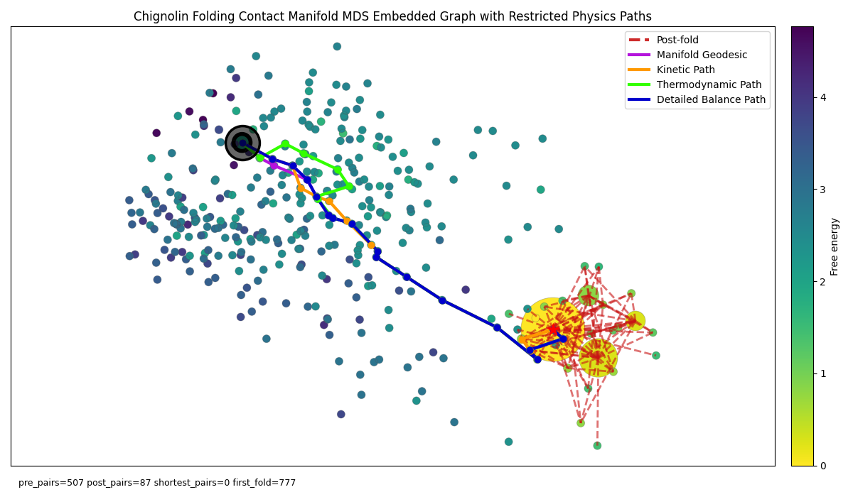Figure 6: Chignolin folding graph with physics-based shortest paths restricted to manifold edges only. Nodes coloured by reweighted Free energy and background edges removed for clarity.

However, if like before, we focus on the manifold geodesic and don’t allow the shortest path algorithm to consider purely temporal edges we encounter a limitation with the current Chignolin trajectory in that most of the manifold edges that underly the long edge temporal edge in the manifold + temporal shortest path are not transitions that are not observed in the trajectory and so have 0 temporal counts and are not weighted in our physics algorithms. Thus the kinetic and thermodynamic paths both converge into the manifold geodesic as it’s the only route to the folded path. If we allow for temporal edges to be seen by the shortest path we get the unrestricted graph: 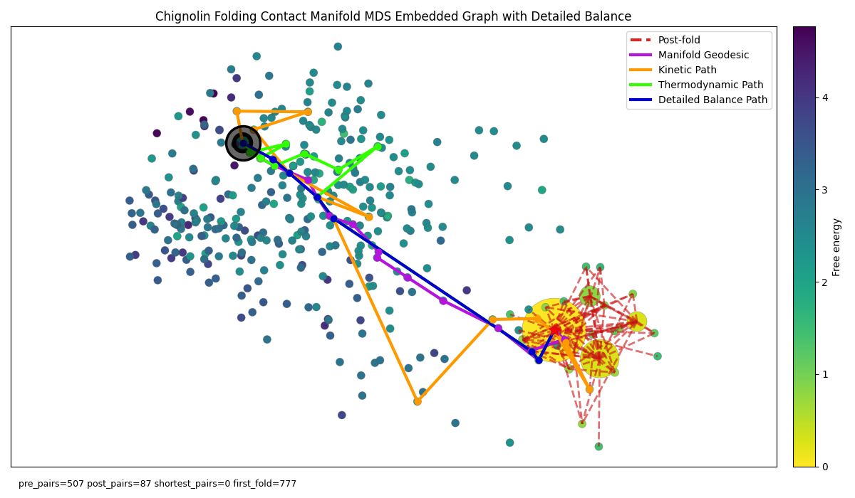Figure 7: Chignolin folding graph with unrestricted physics-based shortest paths (can use manifold and temporal edges). Nodes coloured by reweighted Free energy and background edges removed for clarity.

So when restricted to the manifold edges the paths all converge to the manifold geodesic yet when allowed access to temporal edges we see a significant diversion with the kinetic path, whilst detailed balance nicely recovers the non-physics original shortest path. Does this mean our original non-physics shortest path (or for continuity the manifold geodesic) is a true optimal folding pathway?

Identifying the Transition State Ensemble

Let’s also use another powerful property of graph networks, committor probabilities. Committor probabilities exploit the fact that in graphs we know what possible paths are ahead via node connectivity so at each point we can compute for the probability that node $i$ will reach the folded state before returning to the unfolded state (start node). We’ll exploit something called the Laplacian of the graph which measures how a signal on a node differs from its neighbours. The Laplacian of our graph is given by:

$$ L = D - W $$

Where $D_{ii} = \sum_j W_{ij}$ for all connected nodes $j$, in other words the degree of node $i$. We set the node attribute $q$ such that:

$$ (Lq)_i = \sum_j W_{ij}(q_i - q_j) $$

$$ \sum_j L_{ij}q_j = 0, \quad (Lq)_i = 0 $$

Thus:

$$ q_i = \frac{\sum_j W_{ij}q_j}{\sum_j W_{ij}} $$

Meaning the value $q_i$ for node $i$ is simply equal to the weighted average of its neighbours’ values. We can solve this exactly (for small graphs) given Dirichlet boundary conditions such as those of our shortest path:

$$ q_{\text{start}} = 0, \quad q_{\text{folded}} = 1 $$

Leaving all interior nodes to satisfy $(Lq)_i = 0$. The solution to this bounded Laplacian is the fixed boundary harmonic function of our graph which:

• Provides committor probabilities from Markov-chain theory which is equivalent to a random walk along edges with probabilities proportional to weights
• Minimises the Dirichlet energy which means finding the smoothest possible interpolation between 0 and 1

Hence $q_i$ give us reaction coordinates in the folding pathway and a more rigorous most probable path. With such reaction coordinates we can more explicitly identify the transition state which is canonically defined as the bottleneck of the reaction. If $q=0$ is the probability of unfolding before folding and $q=1$ is the probability of folding before unfolding (folded state) then any node with $q \approx 0.5$ is sitting on the precipice of falling towards either state - imagine it sitting on a ridge tilting into the unfolded and folded energy basins. This will be how we define the transition state ensemble.

Let’s project our graph onto a plot of free energy against reaction coordinates instead of the contact discrete manifold space: 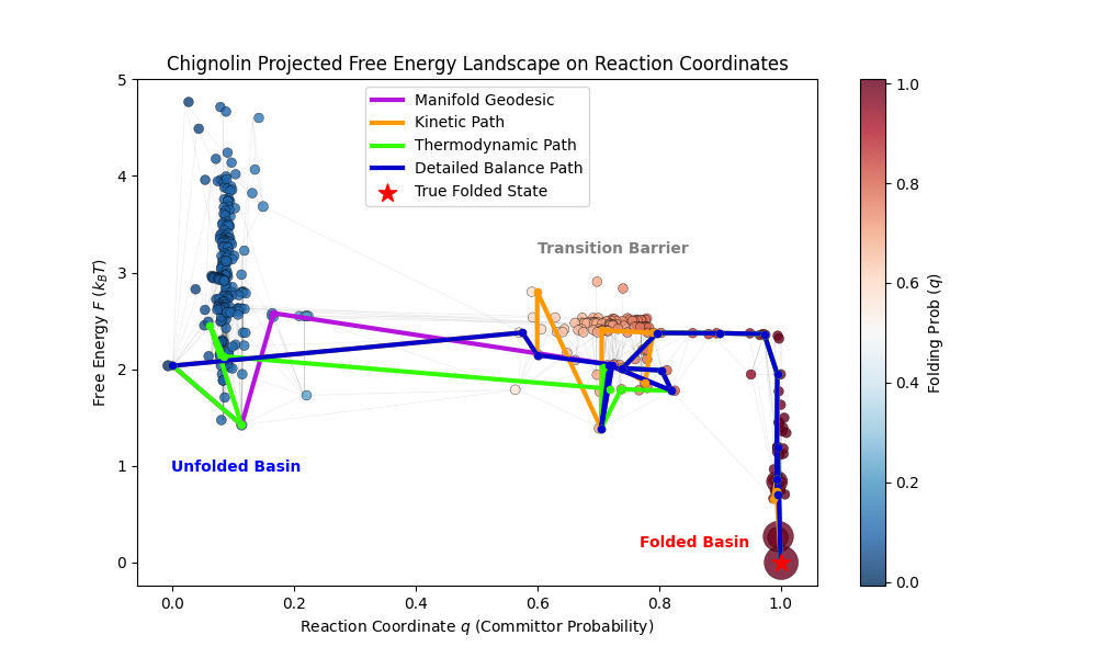Figure 8: Chignolin folding graph projected onto Free energy (y axis) against reaction coordinates (x axis). Node sizes correspond to unique contact map frame counts in the trajectory. The various physics-based shortest paths from before I highlighted and the nodes are coloured by their committor probability.

Note the clear clustering of the different states including the transition state ensemble. This final figure gives us a nice conclusion for Chignolin, it is clearly a downhill folder, as expected from a 10 residue artificial fast folder. For comparison if we take only the first 10% of the trajectory and use the pseudo free energy we get a landscape much more heavily biased by state population counts which leads to a plot more resemblant of a two state folder with stable unfolded and folded states: 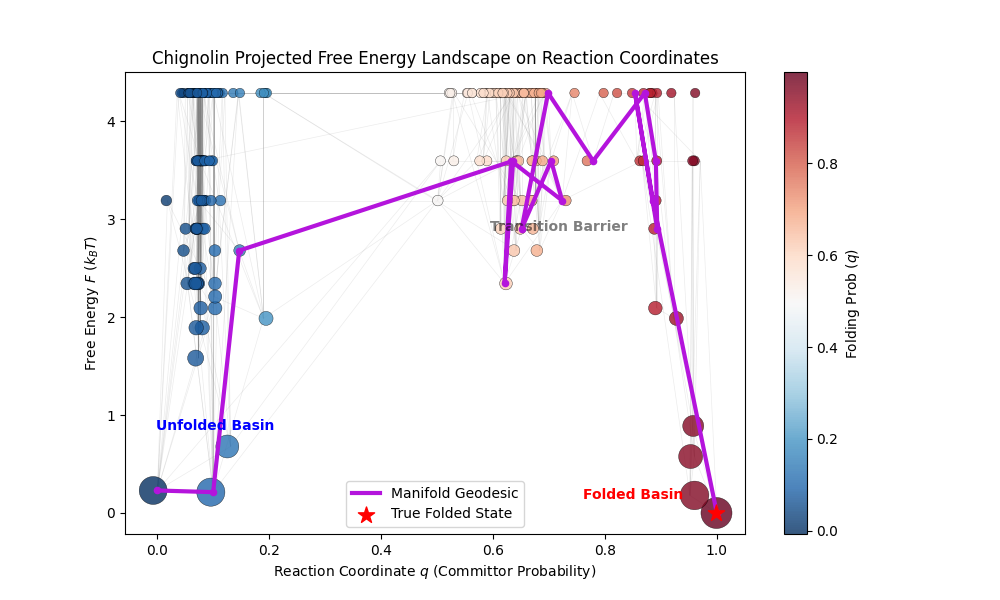Figure 9: Chignolin folding graph projected onto Free energy (y axis) against reaction coordinates (x axis). Only the first 1000 frames of the trajectory (out of 10000) were used and the free energy was computed with the pseudo free energy by Boltzmann inversion and not equilibrium reweighted.

Scaling to Larger Proteins

Although interesting (and pretty), as you may have already concluded this method scales poorly with protein size. The problem is that the number of unique contact maps scales $2^{N_{\text{res}}\choose 2}$ with protein size $N_{\text{res}}$ and so for any reasonably sized protein that is not some artificial fast folder like the 10 residue chignolin in our example the node sizes converge to 1 as the number of possible contact maps vastly exceeds the number of samples (snapshots).

There is a quick but dirty solution. We can cluster contact maps proximal on the manifold of contact space together thus reducing the number of nodes to levels ameanable to data sizes and visualisation requirements. For example, let’s consider the largest protein from the Kresten Lindorff-Larsen et al folding dataset, the lambda repressor. After dimensionality reduction with PCA and UMAP then clustering with HDBSCAN we get the below network (note we don’t use the MDS embedding approach from earlier this time): 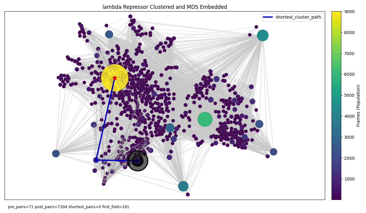Figure 9: Lambda repressor folding graph in the embedded contact map space with nodes representing clusters of unique contact maps close in embedded PCA -> UMAP space. Grey edges connecting temporally adjacent nodes (cluster labels adjacent in the trajectory given each frame in the trajectory is assigned a cluster label). the blue shortest path operates on the temporal edges.

Actually, clustering beforehand is a fundamental step in constructing MSMs (although usually achieved by metrics such as RMSD) as it reduces the number of states to handleable levels but also introduces Markovianity by removing path memory from clustered nodes. Although our shortest path analysis is more fragile as the space of states is too large for continuous manifold edges and temporal edges often traverse unrealistic distances thanks to the clustering we still can perform committor analysis to get reaction coordinates and thus identify transition states: 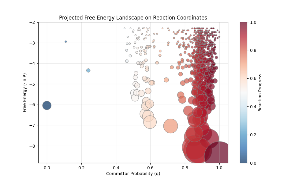Figure 10: Lambda repressor folding graph projected onto Free energy (y axis) against reaction coordinates (x axis). Nodes represent clusters as above and are coloured by their committor probabilities.

Also, although we used unique contact maps as our nodes one could easily employ other state representations such as secondary structure content which would have $4^{N_{\text{res}}}$ configurations as opposed to the contact map $2^{N_{\text{res}}\choose 2}$. Of course in the end we just touched on a number of the practitions used in the more established overarching framework of MSMs.

Take Homes

Despite the limitations forcing us to use a more black box clustering approach, representing protein folding with graph networks becomes a powerful quantitative formalism for geometrically analysing folding pathways across the contact space. Operating in this space has a variety of uses including identifying shortest paths continuous in contact formation/deformation and quantifying the energetic costs of individual contact flips. Grounding our graphs in kinetics shows we can translate this contact map space to a rigorous MSM formulation more standard of MD analysis which we used to identify transition states. If anything else, it was worth the blog post to introduce MSMs but I’ll refer you to more dedicated work for a deeper explanation of these.

Regardless, I’ll keep exploring optimising this for larger proteins and computing the energistic cost contact flips from the graph geometry on the side of my PhD in the limit of data, so stay tuned for future blogs!

The code used in this analysis and links to the MD simulation data is publicly available in the following GitHub repo.