digressions on (mouse) brain imaging - Better MRIcrotome brain outlines

Brain outlines are used routinely in MRIcrotome sliceSeries for showing slice locations, plus they can have value in their own right for replacing the full grey-scale background with an outline. By default the outlines take a bit of trial and error to find the right isointensity lines; in some cases no truly good outlines can be generated. Here I will show an alternate way of generating an outline based on having a hierarchical segmentation present.

1 Setting up

First we’ll load an existing dataset and generate the hierarchical segmentation representations. For those at Oxford using the BMRC cluster you can follow along, for anyone else you’ll have to substitute your own dataset.

First step, read the information about the scans.

library(tidyverse)
gfw2 <- read_csv("exercise-gfw2.csv")

So at this point we have the gf variable containing info about all our files, and gfw2 subsetting them just to the two week timepoint (this is from mice being given access to an exercise wheel).

Next we’ll load the final non-linear average, the segmented final nonlinear average, and build all the volumes.

library(RMINC)

# read the anatomy and labels 
nlin <- mincArray(mincGetVolume("/well/lerch/users/yrf023/plasticity/plasticity-2023-03-10_nlin/plasticity-2023-03-10-nlin-3.mnc"))
labels <- mincArray(mincGetVolume("/well/lerch/users/yrf023/plasticity/plasticity-2023-03-10_nlin/plasticity-2023-03-10-nlin-3/plasticity-2023-03-10-nlin-3_voted.mnc"))

# get all the volumes
allvolsw2 <- anatGetAll(gfw2$labels, defs="/well/lerch/shared/tools/atlases/Dorr_2008_Steadman_2013_Ullmann_2013/mappings/Dorr_2008_Steadman_2013_Ullmann_2013_mapping_of_labels.csv", method="labels")

And now we put the labelled atlas into it’s hierarchy.

# there's a warning that spews everywhere that needs to be fixed in RMINC, but causes no harm.
# so for now I'll suppress these warnings
suppressWarnings({
hdefs <- makeMICeDefsHierachical("/well/lerch/shared/tools/atlases/Dorr_2008_Steadman_2013_Ullmann_2013/mappings/Dorr_2008_Steadman_2013_Ullmann_2013_mapping_of_labels.csv", "/well/lerch/shared/tools/atlases/Allen_Brain/Allen_hierarchy_definitions.json")
hvolsw2 <- addVolumesToHierarchy(hdefs, allvolsw2)
})

2 A basic example

Let’s do a basic example of running a simple linear model, showing it on a brain alongside a slice indicator and legend.

library(MRIcrotome)


Attaching package: 'MRIcrotome'

The following object is masked from 'package:graphics':

    legend

library(grid)

# a simple linear model against group
vs <- mincLm(reljacs ~ group, gfw2, mask = "/well/lerch/users/yrf023/plasticity/plasticity-2023-03-10_nlin/plasticity-2023-03-10-nlin-3_mask.mnc")

Method: lm
Number of volumes: 18
Volume sizes: 161 319 210
N: 18 P: 2
In slice 
 0  1  2  3  4  5  6  7  8  9  10  11  12  13  14  15  16  17  18  19  20  21  22  23  24  25  26  27  28  29  30  31  32  33  34  35  36  37  38  39  40  41  42  43  44  45  46  47  48  49  50  51  52  53  54  55  56  57  58  59  60  61  62  63  64  65  66  67  68  69  70  71  72  73  74  75  76  77  78  79  80  81  82  83  84  85  86  87  88  89  90  91  92  93  94  95  96  97  98  99  100  101  102  103  104  105  106  107  108  109  110  111  112  113  114  115  116  117  118  119  120  121  122  123  124  125  126  127  128  129  130  131  132  133  134  135  136  137  138  139  140  141  142  143  144  145  146  147  148  149  150  151  152  153  154  155  156  157  158  159  160 
Done

# show it as a 3 by 3 slice series
sliceSeries(nrow=3, ncol=3, begin=60, end=250) %>%
  anatomy(nlin, low=700, high=1400) %>%
  overlay(mincArray(vs, "tvalue-grouprunning"), low=2, high=6, symmetric=T) %>%
  legend("t-statistics") %>%
  contourSliceIndicator(nlin, levels=c(700, 1400)) %>%
  draw()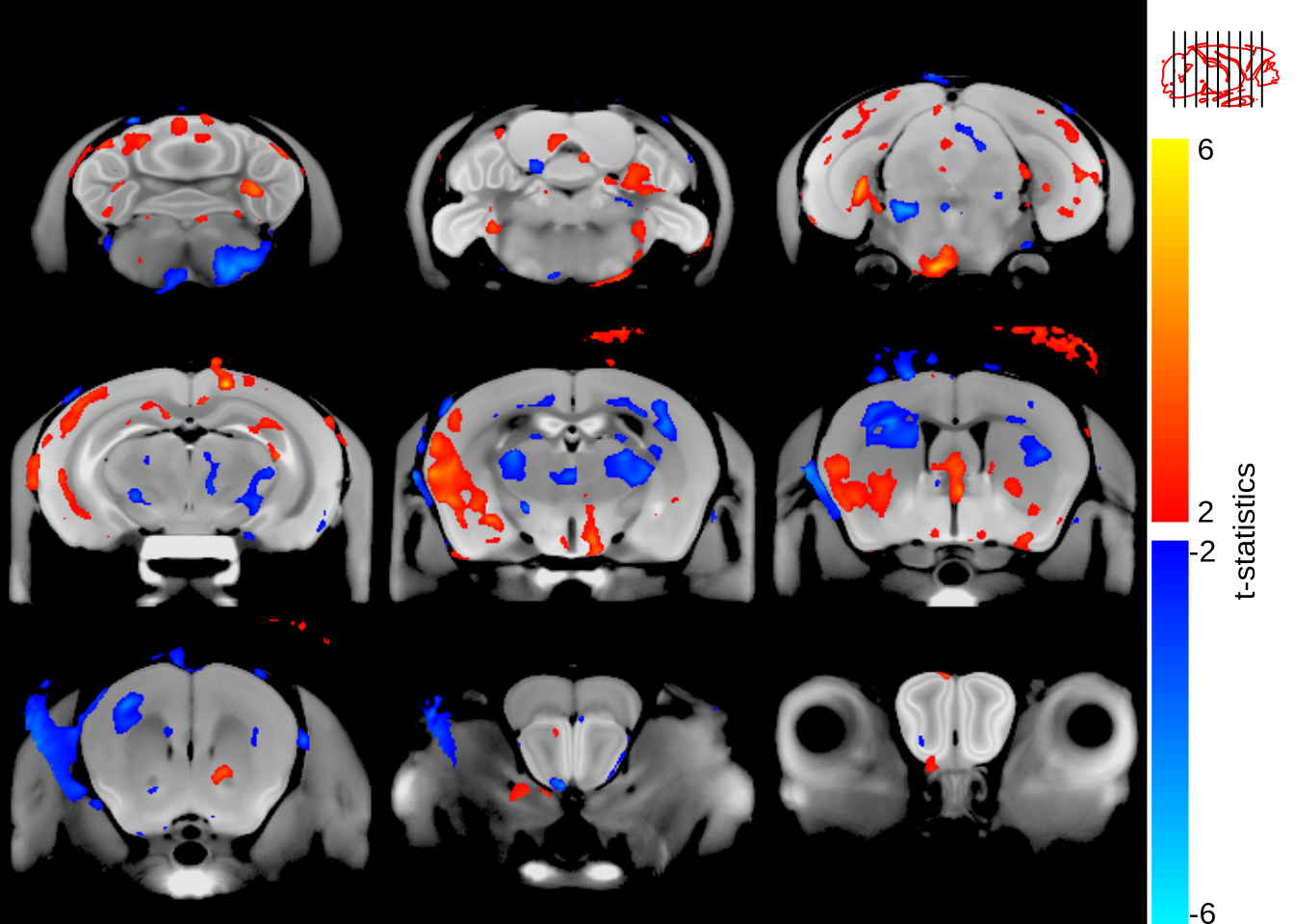

So that looks roughly right - the slice indicator, at the top right, gives a pretty good idea of where the brain is located. But it’s not great; let’s try a few different contours to see what might look better.

sliceSeries(nrow=3, ncol=3, begin=60, end=250) %>%
  anatomy(nlin, low=700, high=1400) %>%
  contours(nlin, levels=c(700, 900, 1100, 1400), col = c("red", "green", "blue", "purple")) %>%
  draw()

Lots of fiddling could be done getting the exact right intensity contours, but it’ll be a challenge to get it just right.

3 Contours based on segmentations

So here’s the trick - the perfect outline is inherently in our segmentation. First, let’s view the segmentation

sliceSeries(nrow=5, ncol=1, begin=60, end=250) %>%
  anatomy(nlin, low=700, high=1400) %>%
  addtitle("anatomy") %>%
  sliceSeries() %>%
  anatomy() %>%
  overlay(hanatToVolume(hvolsw2, labels, "color_hex_triplet"), low=0, high=1) %>%
  addtitle("segmentation") %>%
  draw()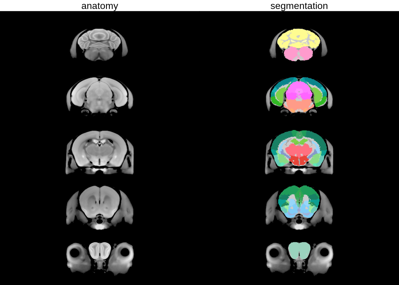

Now the key part here is that the labels are in a hierarchy. A clean outline could thus be taken if we use just the first parts of that hierarchy:

library(data.tree)
# create a copy of the hierarchical tree
hdefs2 <- Clone(hvolsw2)
# and prune it to just the first four levels 
hdefs2$Prune(function(x) x$level<4)

Warning: 'hdefs2$Prune' is deprecated.
Use 'Prune(node, ...)' instead.
See help("Deprecated")

[1] 495

# print it to see what it looks like
print(hdefs2, limit=Inf)

                                               levelName
1  root2                                                
2   <U+00A6>--Basic cell groups and regions             
3   <U+00A6>   <U+00A6>--Cerebrum                       
4   <U+00A6>   <U+00A6>--Brain stem                     
5   <U+00A6>   <U+00B0>--Cerebellum                     
6   <U+00A6>--fiber tracts                              
7   <U+00A6>   <U+00A6>--cranial nerves                 
8   <U+00A6>   <U+00A6>--medial forebrain bundle system 
9   <U+00A6>   <U+00A6>--cerebellum related fiber tracts
10  <U+00A6>   <U+00A6>--lateral forebrain bundle system
11  <U+00A6>   <U+00B0>--extrapyramidal fiber systems   
12  <U+00B0>--ventricular systems                       
13      <U+00A6>--cerebral aqueduct                     
14      <U+00A6>--fourth ventricle                      
15      <U+00A6>--lateral ventricle                     
16      <U+00B0>--third ventricle

Now create an outline based on this pruned hierarchy

sliceSeries(nrow=5, ncol=1, begin=60, end=250) %>%
  anatomy(nlin, low=700, high=1400) %>%
  sliceSeries() %>%
  anatomy() %>%
  overlay(hanatToVolume(hvolsw2, labels, "color_hex_triplet"), low=0, high=1) %>%
  sliceSeries() %>% anatomy() %>%
  contours(hanatToVolume(hdefs2, labels, "position"), levels=c(0.5, 1.5, 2.5, 3.5), col="red") %>%
  draw()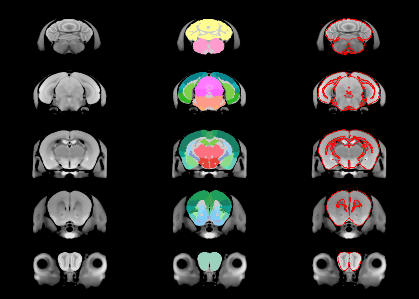

And there you have an almost perfect outline of the brain. So let’s recreate that earlier figure with the cleaner outline:

sliceSeries(nrow=3, ncol=3, begin=60, end=250) %>%
  anatomy(nlin, low=700, high=1400) %>%
  overlay(mincArray(vs, "tvalue-grouprunning"), low=2, high=6, symmetric=T) %>%
  legend("t-statistics") %>%
  contourSliceIndicator(hanatToVolume(hdefs2, labels, "position"), levels=c(0.5, 1.5, 2.5, 3.5)) %>%
  draw()

Voila.