Data Analysis for Neuroscientists IV:
Sample vs. Population

Island of Shetland - population 22,210

The population Last week we generated a simulated height 'dataset': h - drawn from a Normal distribution with mean 179cm and standard deviation 7cm These are the true statistics for British men Shetland is an island to the North of Scotland with a population of 22,210 and some impressive weather. Generate a vector with simulated heights for 10,105 men (let's call this the entire male population of Shetland) with these statistics. HINT Remember you can do this using the function randn which generates normally-distributed random numbers with a mean of 0 and a standard deviation of 1, with some small modifications

Heights of Shetland Men

The sample

Whilst out walking on Shetland, I encounter our old friend Eric, with a group of 5 men.

From their height, I suspect they are not from around here. They seem to be a little taller than the local men.

Also, I don't like the look of them.

How can I determine whether these are bone fide Shetlanders or possibly an invading army?

Simulating samples from the null population

One way we can work out if Eric and his friends really belong to the local population is:

• find the mean height of my test group (Eric et al)


• draw lots of samples of size 5 from the true local population


• how often do I get a group whose mean height is as tall as Eric and co?
• if this is very unusual, we may conclude that Eric and co are not as local as they claim to be

Let's explore what happens if we draw samples of 5 men from our population.

First, let's draw one random sample of 5 men from our population by:

• Creating an index vector ix with random numbers between 1 and 10,105
• Using it to pull out the heights of the indexed men into a new vector, s (for sample)
• Finding the mean m of the sample

?

First make an index vector with random numbers between 1 and 10,105

>> ix = randi(10105, 5, 1)

Now get the heights of the indexed men

>> s = h(ix);

and find their mean

>> m = mean(s);

Now we are going to draw 1000 samples of 5 men each from the population of Shetlanders.

• Make a for loop to do this

?

>> for i = 1:1000
>>     ix = randi(10105, 5, 1)
>>     s = h(ix)
>>     m(i) = mean(s) % note I am now saving the means into a vector with 1000 entries
>> end;

• Plot a histogram of the sample means for the samples of 5 men

?

>> hist(m,50) % histogram with 50 bins

• The histogram show the distribution of the sample mean, m, for samples of size 5

?



• What is the mean of the distribution of means?

?

>> mean(m)

• How does this compare to the mean height of the population of Shetlanders?
• What about the standard deviation of the distribution of mean?

?

>> std(m)

• The mean height of Eric's group was 184 cm.
  What % of our samples of 5 true Shetlanders are at least as tall as Eric's group?

  HINT

  Use find

  Go on, tell me!

  >> tall_ix = find(m>=184)
  >> length(tall_ix)

  I make it about 6% of samples of n=5 that are taller than Eric and co.

Notice something really important here: by working out the null distribution of the sample mean we were able to put a number on how unlikely it was that the test sample (Eric and co) were drawn from the null distribution (the population of Shetlanders).

?

We can think of this in hypothesis testing terms:

• The null hypothesis H₀ is that Eric and co are a random sample of
  • n=5 Shetlanders with
  • mean height 179 cm
  • sd 7 cm
• The alternative hypothesis H₁ is that they are Bloodthirsty Viking Invaders!!
• To find out how unusual the mean height of Eric's group is, we need to know the distribution of means that we would get if we drew samples of size n=5 from the null population (Shetlanders) many many times
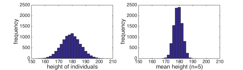
• This sampling distribution of the mean is not the same as the distribution of individual heights

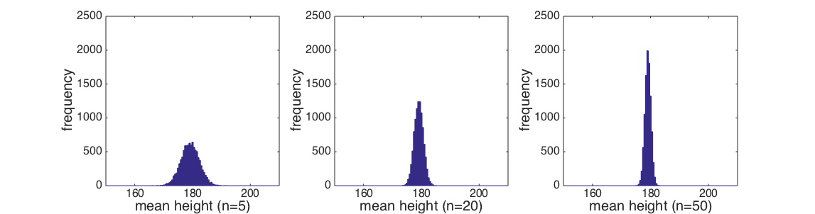
The effect of sample size

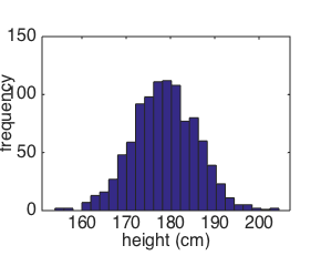
The mean height of Eric's group was unusual - if we draw samples of 5 men from the population of Shetlanders, about 6% of those groups would be as tall as Eric and co.

However this would not pass a test of statistical significance - usually a sample woud be considered significantly different from the null population if it would have occurred less than 5% (or 1% or 0.1%) of the time due to chance.

What if some more of Eric's friends now show up, so we now have a test sample of 20 possible Viking Invaders with mean height 184 cm. How likely was this under the null hypothesis?

• Work it out by simulation as we did for samples n=5

?

• Modify the previous for loop to generate 1000 samples of size 20
• How many of these have a mean of at least 184cm?

What about samples of size 50?

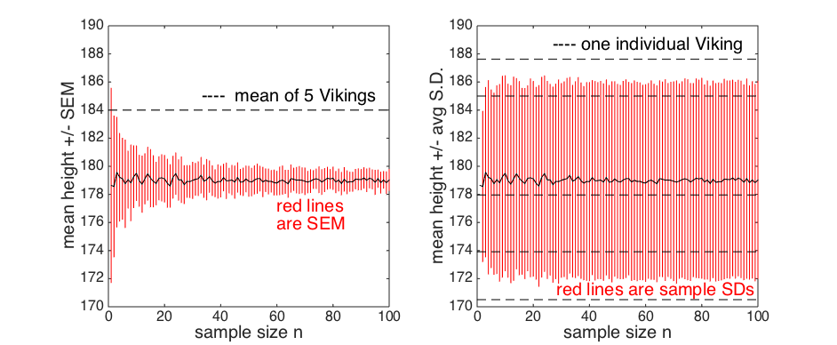
Standard error of the mean (SEM)

We have seen that the larger the sample, the tighter the distribution of the sample mean.

This makes intuitive sense as, if the deviation of the sample mean from the population mean was just due to chance (ie, I happen to have picked unusually tall Shetlanders), the more people I put into my sample, the less likely it is that they are all tall guys.

The relationship between sample size, and the spread of the sample means we get if we run lots of samples, is captured by the following equation Careful! if you are using Chrome the sqrt sign here is invisible! please use Firefox!:

SEM =	s
	$\sqrt{n}$

... where s is the sample standard deviation, n is the number of data points in the sample, and SEM stands for the Standard Error of the Mean

The Standard Error of the Mean is none other than the standard deviation of the distribution of sample means, for a given sample size n - the spread of the different distributions plotted at the top of this section.

We are not going to prove mathematically that the SEM is inversely proportional to $\sqrt{n}$, but the result is so important that it is worth checking it by simulation.

Can you adapt the script you made earlier, so that it generates 50 samples each of size 1,2,3,...100 (note 50 and not 1000 samples - those MSc Centre computers may explode if you make 1000 samples each for 100 values of n!), and records their sample means and standard deviations?

HINT

You already know how to make a for loop that generates 50 samples for a fixed n, eg n=5 or n=20

You need to embed this in an extra for loop, which runs your old for loop for each value of n from 1 to 100

?

>> n=1:100
% list of sample sizes to be tested
>> for j=1:length(n) % counter variable for outer loop
>>     for i=1:50
>>         ix = randi(10105,n(j),1);
>>         s = h(ix);
>>         mm(i,j) = mean(s);
>>         ss(i,j) = std(s);
>>     end
>> end

Note that the output matrices mm and ss are now two dimensional:

• Each column corresponds to a sample size n
• The 50 rows are the 50 samples for each size n
• So there are two counter/indexing variables -
  • i counts out the 50 samples for each value of n and is the row index for the output matrices
  • j counts out the 100 values of n and is the column index for the output matrices

Then we can plot the standard deviation of the sample means, that is the SEM, against n

?

>> n=1:100
>> sem = std(mm)
>> plot(n, sem)

And add a line showing the theoretical value of SEM from the formula above for each n, for comparison:

?

>> hold on
>> sem = 7./sqrt(n)
>> plot(n, sem, 'r')

By the way, I've cheated here and assumed that the sample standard deviation is about 7 - the population standard deviation.

Since the SEM is usually calculated for a single sample, we would normally be working with a single sample standard deviation.

Is it a good match?

Standard error vs. Standard Deviation

To recap: how unusual a sample is, given the null population, depends on

• The distance of the sample mean from the population mean
• The square root of the sample size: $\sqrt{n}$

... and we determine whether a sample of n observations (men in this case) differs from the population by considering the distribution of sample means if we drew many samples from the null population - we do not compare the mean of the sample to the null population itself but to the distribution of sample means for samples drawn from the null distribution

An aside...

Does the variability within the sample (the sample standard deviation) also depend on n?

• When we generated all those samples with different values of n,
  we saved the sample standard deviations as well as the sample means,
  in a matrix called ss
• Now plot the mean sample standard deviation for each n against n

?

>> n=1:100
>> mean_ss = mean(ss)
>> plot(n, mean_ss)


No, the sample standard deviation does not vary with n

It is the SEM, not the sample SD, that tells us how unusual our sample is.

The central limit theorem

The distribution fo sample means looked approximately Normal for our height data.

Perhaps that was not surprising given that the height data themselves were Normal.

But one of the most powerful results in statistics is that:

• For any data distribution...
• ... the distribution of the sample mean is approximately normal
• ... as long as the sample is large enough
• ... and it doesn't have to be that large

This result is called the Central Limit Theorem and can be proved mathematically but we are not going to do that now.

Instead we are going to prove it to ourselves using simulation.

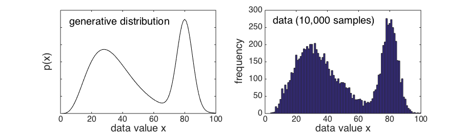
Some very non-Normal data

Download the data file "nonNormalData.txt" which contains 10,000 samples from this distribution, and load it into Matlab as a vector called data

These data are very non-Normal, in fact they are bimodal (there are two peaks)

However, the Central Limit Theorem tells us that if we draw samples from this distribution, their sample means with be Normally distributed, as long as the samples are large enough.

Let's try it for a very small sample size, n = 2.

• Make a for loop to draw 10,000 samples of size n = 2 from the distribution
• For each sample work out the sample mean
• Then plot all the sample means in a histogram

?

I think you might be able to do this yourself based on what we did earlier.

TELL ME!

>> for i=1:10000
>>      ix = randi(10000, 2, 1)
>>      s = data(ix)
>>      m(i) = mean(s)
>> end
>>
>> hist(m,[1:2:100]) % the [1:2:100] tells it which bins to use for the histogram


• Probably the distribution of sample means didn't look very normal for n = 2
• In fact if you look closely you may notice that it has 3 peaks, corresponding to the cases where:
  • both samples came from the left hump of the data distribution
  • both samples came from the right hump of the data distribution
  • one came from each

But what happens if I go for a slightly larger sample, n = 5 or n = 10 ?

• Repeat the previous exercise for n = 5 and n = 10
• Is the distribution of sample means starting to look Normal?

In practice, the approximately Normal distribution of the sample mean emerges from even very non-Normal data distributions with quite small values of n

As n tends to infinity, the distribution of the sample becomes exactly Normal.

SEM for non-Normal data

What about the spread of the distribution of sample means?
Does the relationship to $\sqrt{n}$ hold even for very non-Normal data?

• Repeat the exercise above in which we:
  • Generated 50 samples of size n for n=1:100
  • Plotted the standard deviation of the sample means (ie, the SEM) as a function of n
  • Added a plot of 1/$\sqrt{n}$ to the plot
• Does the relationship hold?

Hopefully you should have found that the standard deviation of the distribution of sample means, which is exactly the SEM, is inversely proportional to $\sqrt{n}$ even for highly non-normal data.

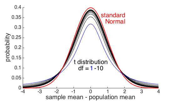
The t-distribution (a special case)

The Central Limit Theorem tells us that when n is large, the null distribution of sample means is (very) nearly Normal.

As we have seen, when n is small, the shape of the distribution of sample means depends on the data distribution.

For Normally distributed data, there is a known, precise distribution for the sample mean for any value of n

• The distribution of the sample mean for Normal data is the t(df) distribution
• df stands for degrees of freedom and is given by: df = n-1

As you can see from the picture above, the t distribution has heavier tails and a pointer point than the Normal distribution. These features together are sometimes called positive kurtosis

Remember that the probability of an observation happening due to chance if given by the area under to curve to the right of the point on the x-axis corresponding to the observation.

For example, say the sample mean is 3 standard errors from the population mean and n=5.

• Use normcdf to work out how often this would happen due to chance if the sample mean followed the standard normal distribution (which it would if n was large)

• ?

  >> normcdf(3,0,1)
  

• Use tcdf to work out how likely this actually is for n=5

?

>> tcdf(3,4) % Careful, df is n-1 not n

Although the t-distribution and the Normal distribution look quite similar, they differ in the crucial region for determining statistical significance (ie, the tails)

For a small sample size n=5, an extreme observation 3 SEMs from the population mean is over 10x as likely (based on the t(4) distribution) as we would predict if we assumed the sample mean exactly followed the Normal distribution.

So if the data are Normally distributed then we can work out exactly how unlikely the sample mean was even for small n, using the t-distribution

Extra exercises (advanced)

Generating samples from an arbitrary distribution

How did I generate the non-normal data above?

First, I made a arbitrary probability generating function

>> x = 1:100;
>> px = normpdf(x,80,5)/2 + gampdf(x,5,7)
>> px = px./sum(px) % force the distribution to integrate to 1

Then, I generated 10,000 uniform distributed random numbers

>> u = rand(10000,1);

Then I used a probability integral transform to convert these to my desired probability distribution:

• For each if my uniform samples u(i), the probability of drawing another sample from the uniform(0,1) distribution that is bigger than u(i), is simply u(i).
• There must be some value of x such that the probability of drawing a sample from p(x) that is greater than x, is equal to u(i)
• x and u(i) are said to be probability matched
• Replace each value u(i) with the probability matched value of x to get samples from p(x)

>> for i=1:length(u)
>> data(i) = x(find(cumsum(px) > u(i),1));
>> end

Can you see how this relates to the last section of last week's work on the probability integral transform?

Make your own probability distribution (try a trimodal one) and generate some data from it.