Data Analysis for Neuroscientists V:
Regression

Subject recruitment, 1904 style, at the Galton Lab (notice the subject pays the experimenter!)

Regression: How to predict one variable from another variable

Last week looked at how to test for differences between sets of data points - eg between the heights of alleged Vikings and bone fide Shetlanders.

This week we will consider a complementary question:

How can the value of one variable be predicted from the value of another variable?

For example:

• How can the firing rate of a retinal receptor cell be predicted from the intensity of light falling on it?
• How can the activity of a brain region (measured with fMRI) be predicted from the difficulty of the arithmetic problem being solved at the time?
• How can a participant's choices in a gambling task be predicted based on the magnitude of the expected payout?

All of these questions can be addressed by fitting regression models.

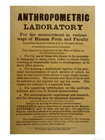
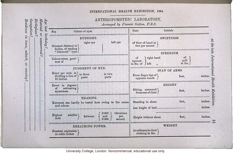
Galton's measurements: child vs. midparent In the early 20th Century, Galton set up his "Anthropometric Laboratory" in which he measured a whole set of characteristics of individuals (including, notably, collecting some of the first reaction time measurements) He got a lot of data and people actually paid to take part in his study (see handbill above)! One of Galton's observations was that children's height is similar to the average of their parents' heights (the 'midparent height') Download Galton's data parentChildHeight.txt Load it into Matlab as a matrix called heights Each row is one child. Column 1 is the midparent's height (mean of father and mother's height) Column 2 is the child's height Heights are in inches and are rounded to the nearest inch Plot the childrens' heights against the midparent heights ? >> plot(heights(:,1),heights(:,2),'o')

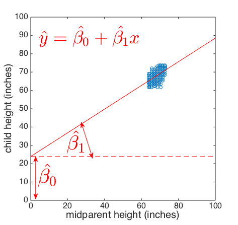
Fitting the regression line The red line on the graph above is a regression line, indicating the best fit linear relationship between: Our explanatory variable: midparent height also called the independent variable plotted on the x-axis often manipulated by the researcher (but not in this case) Our response variable: child height also called the dependent variable plotted on the y-axis observed but not manipulated by the researcher The simplest case is that the predicted value $\stackrel{}{^}$ of the dependent variable y is a linear function of the independent variable x $\stackrel{}{^}=\; mx\; +\; c$ We tend to use slightly different notation: $\stackrel{}{^}$ = $\stackrel{}{^}$1x + $\stackrel{}{^}$0 .... where $\stackrel{}{^}$0 is the estimated y-intercept and $\stackrel{}{^}$1 is the estimated gradient. We can find the values of β0 and β1 analytically (using an equation) but we are not going to go into the mechanics of this today. Instead we will fit the regression line using the Matlab function glmfit Use glmfit to find the values of $\stackrel{}{^}$0 and $\stackrel{}{^}$1 ? >> b = glmfit(heights(:,1),heights(:,2)) What is the fitted slope? What is the fitted y-intercept You can work out which is which either from the help info, or by common sense Add a regression line to your plot using these values ? You need to specify some sensible x-axis values >> xvals = 62:74 ... and the fitted y-axis values >> yhat = b(1) + b(2).*xvals ... and then plot them >> hold on >> plot(xvals,yhat,'r');

The Residuals

The difference between the fitted data and the actual data, $\stackrel{}{^}$ - y, are called the residuals

When fitting the regression line we chose values of $\stackrel{}{^}$₀ and $\stackrel{}{^}$₁ to minimise the square of the residuals (this is called "ordinary least squares" regression, or OLS).

OPTIONAL MATHS: WHY minimize squared errors?

One answer that is often given is that if we square the residuals, we are treating positive and negative errors (data points above and below the regression line) as equivalent, and only considering the size of the errors. Why not then just minimize the absolute errors?

Actually, the real answer comes from the fact that the data points are supposed to be Normal distributed about the regression line. The equation for probability of y under a normal distribution with some mean, $\stackrel{}{^}$, and standard deviation σ is:

Now, you can see that the probability of the data points given some regression line depends on the square of the distance of the actual data points y from the points predicted by the regression line, $\stackrel{}{^}$. So the regression line that had the highest likelihood of producing thoe observed data points, is the one for which ($\stackrel{}{^}$ - y)² is minimized.

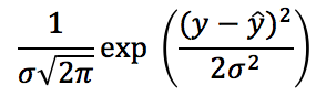
We can find the residuals for our regression by working out the predicted value of child height y, that is, $\stackrel{}{^}$, for each value of midparent height x in our data set...

?

>> yhat = b(1) + b(2).*heights(:,1)

... and then doing $\stackrel{}{^}$ - y

?

>> res = yhat - heights(:,2)

Plot a histogram of the residuals. Are they normally distributed?

?

Not so much. At least if you use plenty of bins (~50) you can see this. One problem is that the data are heavily rounded (to the nearest inch, even though the range is only about 12 inches).

Testing, testing

The regression line for the data we just generated looks pretty convincing. But how can we test if the relationship is statistically significant?

To test whether there is a significant relationship between x and y, we want to test whether the slope is significantly different to zero. There are two factors that should influence our opinion about this:

• What is the gradient of the slope? If the slope is very flat, we should be more likely to believe that the real relationship could be zero than if the slope is steep.
• How sure are we about the gradient of the slope?

If this second point sounds a bit strange, consider the cases below:

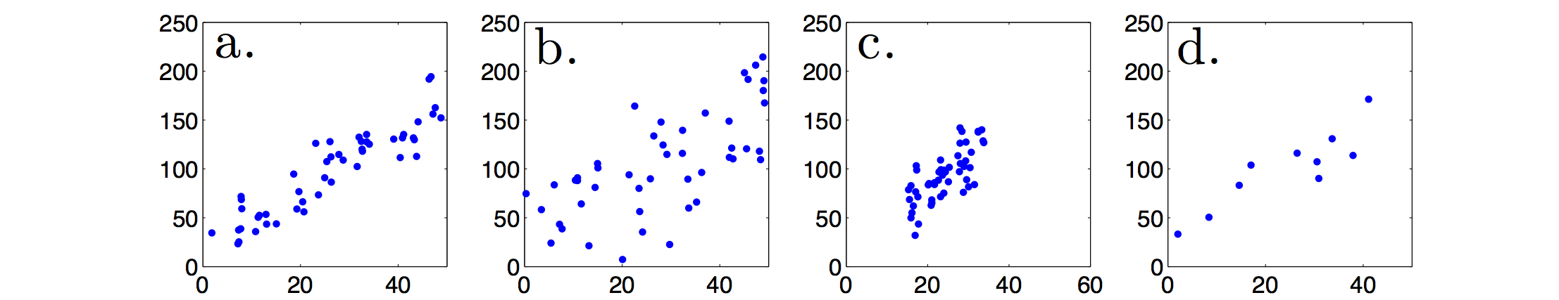
1. Our original data
2. More spread in y --> more uncertainty about slope
3. Less spread in x --> more uncertainty about slope
4. Fewer data points --> more uncertainty about slope

The equation for the standard error (SE) of the regression slope captures all of these factors:

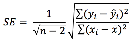
In other words -

• For each data point y_i, the further it is from the predicted value $\stackrel{}{^}$_i, the higher the SE
• For each data point x_i, the further it is from the mean value $\stackrel{}{\_}$, the lower the SE
• The more data points we have (high n), the lower the SE

The significance of the regression slope can then be calculated simply by defining the t-statistic:

t = β1/SE

... where β₁ is the fitted regression slope....

And comparing it against the t-distribution with (n-2) degrees of freedom.

Exercise: significance of the regression slope

To calculate the t-value for our regression:

• Work out Σ(y_i - $\stackrel{}{^}$_i)² using the fitted values and values of y (child height)
• Work out Σ(x_i - $\stackrel{}{\_})2where$ \stackrel{}{\_}$is\; the\; mean\; of\; the\; x\; values\; (midparent\; height)$
• The number of data points n is easy to work out!

?

>> n = length(heights);
>> x = heights(:,1);
>> y = heights(:,2);
>> yhat = b(1) + b(2).*x % Careful, we found yhat earlier but not for these values of x!
>> SE = (1./sqrt(n-2)).*sqrt(sum((y-yhat).^2)./sum((x-mean(x)).^2));
% careful with brackets here! you want to first square x-mean(x), then do the sum of it - not vice versa!
>> t = b(2)/SE;
>> p = 1 - tcdf(t,n-2); % why 1-tcdf? because we want the upper tail of the t distribution

Then we get the p-value by comparing to the t(n-2) distribution

?

>> p = 1 - tcdf(t,n-2); % why 1-tcdf? because we want the upper tail of the t distribution

Exercise: Standard error of the regression slope

What does it mean to talk about the Standard Error for a slope, actually?

Last week, we looked at the Standard Error of the Mean (SEM) for samples:

• The SEM is the standard deviation of the distribution of the sample mean.


• So when we...
  
  • generated lots of samples (say, samples of 10 Normal-distributed random numbers)
  • found the mean of each sample,
  • plotted a histogram of those means
  
  ...the spread of that histogram was what was captured by the SEM.

In other words, the SEM for the sample tells us about the spread of our estimate of the sample mean - which is important if we want to say whether the difference between the sample mean and some reference value (like a population mean, or zero) could have arisen due to chance.

The SE of the regression slope, similarly, tells us about a distribution of possible slopes that we might have got, if we had sampled different data from the same distribution

To get a feel for this, let's try grabbing smaller samples from our 'population' of 928 children and running the regression on them, then plotting all the resulting regression lines on the same graph to see how the slope varies:

• Can you make a script with a for loop that:
  
  • generates 100 samples of size 50 from the population
  • finds the regression coefficients for each sample
  • saves them into a matrix
  • plots the relevant regression lines
  
  
• It may help to look back at last week's work



?

n=100;
figure;
plot(heights(:,1),heights(:,2),'o');
hold on;

for i=1:100 % 100 samples
     % fit the regression
     ix = randi(length(heights),n,1);
     s = heights(ix,:);
     b(i,:) = glmfit(s(:,1),s(:,2));
    
     % plot it
     xvals = 62:75;
     yvals = b(1,i) + b(2,i) .* xvals;
     plot(xvals,yvals,'r');

end;

% add a line representing the null hypothesis of no relationship
ymean=mean(heights(:,2));
plot(xvals,ones(size(xvals)).*ymean,'k','LineWidth',2);


• Now do it again for samples of size 10.
  • Did the distribution of slopes gets smaller?
  • How should the standard error have changed (look at the formula)

Take home message

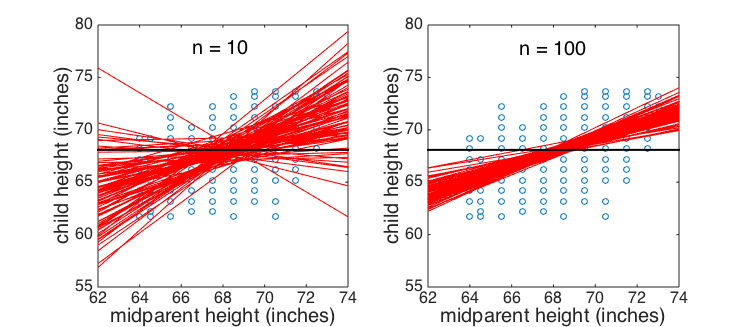
Regression slopes based on samples of 10 and 100 subjects from the same subject population

Although the statistic we are looking at is different from last week (a sample regression slope rather than a sample mean), to work out whether an effect is significant, we are considering how frequently an event would happen (in this case, how frequently some value for the regression slope would be above zero) if we repeated the experiment lots of times.

Further Exercises

Look back at the Oxford Weather data from the 2nd class. There is clearly a relationship between temperature and month - but it is not a straight line. How can we fit this with regression?

HINT: it looks sinusiodal to me...