Correlation and Covariance

In the past couple of weeks we have been looking at linear regression - predicting the value of a response (dependent) variable from the known values of some explanatory (independent) variables.

This week we are looking at a related concept - correlation - and its close cousin covariance.

Hopefully by the end of this class everyone will know the difference between (and relationship between) regression, correlation, and covariance.

Variance and covariance

Say I measure the length and weight to 100 rats and plot them on a scatter graph. Load the data file rats.txt and plot the data with one dot per rat, length in cm on the x-axis, and weight in grams on the y-axis.

• Would you say there is a relationship between the length and weight of the rats?
• What is the variance of the lengths of the rats?

  ?

  Variance is standard deviation squared. But you could also use the formula:

  $\mathrm{V(X)}=\; \Sigma \; (x-\stackrel{\_}{x})2$

  ... Where V(X) is the variance of X and $\stackrel{\_}{x}$ is the sample mean.

• What is the variance of the weights of the rats?
• Do these two variances capture the joint distribution of heights and weights?
  Generate 1000 "rat" samples, each with a height and weight, such that:
  • The lengths are Normal distributed with the mean and variance matching the sample mean length and sample lengths' variance.
  • The weights are Normal distributed with the mean and variance matching the sample mean weight and sample weights' variance.
  ... and plot the samples on a scatter plot

  ?

  >> m = mean(rats) % get the sample mean length and weight for the rats in the text file
  >> s = std(rats)
  >> sim_rats(:,1) = m(1) + randn(1000,1).*s(1) % Normal-distributed "lengths" for 1000 rats
  >> sim_rats(:,2) = m(2) + randn(1000,1).*s(2) % "weights"
  >> figure; plot(sim_rats(:,1),sim_rats(:,2));

• Do you see the same relationship between length and weight as we had in the original sample?

  ?

  No, there is no relationship between height and weight in our simulated data, because we generated the heights and weights independently without modelling the relationship between them.

What we need to know to capture the relationship between length and weight is not just the variance of length and the variance of weight, but how much they covary

The formula for covariance is as follows:

$\mathrm{COV(X,Y)}=\; \Sigma \; (x-\stackrel{\_}{x})(y-\stackrel{\_}{y})$/(n-1)

There is a clear analogy with the formula for variance:

$\mathrm{V(X)}=\; \Sigma \; (x-\stackrel{\_}{x})2$ = Σ $(x-\stackrel{\_}{x})(x-\stackrel{\_}{x})$/(n-1)

In other words, V(X) = COV(X,X).

Whilst the variance tells you about how spread out the data are along one dimension, the covariance tells you whether the spread in more than one dimension is related.

If values of x that are a long way from the mean of x tend to be paired with values of y that are a long way from the mean of y, then the covariance will be large

• Look at the plot of length against weight for the rat data from the text file. Identify some rats that are a long way from the mean in weight. Are the lengths of these rats also a long way from the mean?
• What about the simulated data we made using randn ?

The covariance matrix

For the original sample of rats (in the text file) work out the covariance between their lengths and weights using the formula above

?

>> m = mean(rats)
>> cov_xy = sum((rats(:,1) - m(1)).*(rats(:,2) - m(2)))/(length(rats)-1)

Wot?? Let's unpack that...

>> x = rats(:,1) % lengths in 1st column
>> y = rats(:,2) % weights in 2nd column
>> mean_x = mean(x)
>> mean_y = mean(y)
>> n = length(rats)
>> deviations = (x-mean_x).*(y-mean_y)
>> cov_xy = sum(deviations)/(n-1);

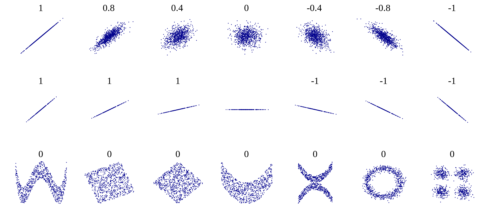
The variance and covariance for two-dimensional data sets (like the length/weight data) can be summarised in a covariance matrix, which is often (confusingly!) called Σ:

Work out the covariance matrix for the length and weight of the rats, using the formulae for variance and covariance.

You can also get MATLAB to work out the covariance matrix for you using cov. Use this function to check your covariance matrix.

?

>> cov(rats(:,1),rats(:,2));

Variance and covariance depend on the data range ...

Imagine I had measured the rats' lengths in mm instead of cm. What would the covariance matrix look like in this case?

• Use the formulae for variance and covariance to find the new covariance matrix, having multiplied the lengths by 10 to put them into mm from cm.

Hopefully, you should have found that the variance of the lengths and the covariance of length and weight, changed.

Note that the underlying relationship between lengths and weights should be the same regardless of the measurement units. And if you were to plot the lengths in mm against the weights, the only change in the appearance of the graph would be the labels on the weight axis.

Importantly, the key thing that covariance is supposed to capture (that extreme values of length and weight tend to co-occur in the same rats) is still just as true as ever.

... but correlation does not

In cases where we are interested in how tight the relationship between variables x and y is, but not necessarily in how much x and y themselves vary, we can use a from of covariance that is normalised for the variance of x and y.

$r$ = (1/n-1) Σ $(x-\stackrel{\_}{x})\; (y-\stackrel{\_}{y})$ / σ_xσ_y

Where σ_x and σ_y are the standard deviations in x and y.

This normalised covariance measure, r is in fact the correlation between x and y.

• Work out the correlation beween length in cm and weight for the rat data
• Do the same using length in mm. Hopefully, unlike the covariance, the correlation should be insensitive to the units of length
• Make the correlation matrix between rats' length and weight using the formula above.
  • In the covariance matrix we have the variance of X (or Cov(X,X)) and variance of Y on the main diagonal.
    
  • What will the elements on the main diagonal of the correlation matrix be?

    ?

    The correlation of X with itself and the correlation of Y with itself - which will both be 1.

• Check your correlation matrix is the same as the one you get using the MATLAB function corr.

  ?

  >> corr(rats)

Correlation is independent of the regression slope

As we just saw, the correlation between X and Y is the ratio of the covariance of X and Y to the variance in X and Y.

We can change the range of one variable by a factor fo 10 (by writing the rats' lengths in mm instead of cm) and the correlation doesn't change.

Let's just think for a minute about the equivalent situation if we were doing a regression. Say we want to regress the rats' weights on their lengths:

?

>> b_cm = glmfit(lengths_cm, weights)
>> b_mm = glmfit(lengths_mm, weights)

The regression coefficients, b_cm and b_mm, are quite different - because the regression coefficients predict the rat's weight from its length in either cm or mm, and the number we need to multiply the length in cm by to predict the weight of a rat of a certain length is 10x larger than the number by which we would multiply its length in mm.

But as we just saw, the correlation is the same for lengths in cm or mm.

This highlights a key but often misunderstood point about the interpretation of correlations:

• The correlation coefficient does not tell you anything about the slope of the line (apart from whether it is positive or negative).
• The correlation coefficient is purely a measure of how tight the relationship between X and Y is.
• A high correlation coefficient does not mean that a change in x translates to a big change in y. It only means that the value of x reliably predicts the value of y.

To labour the point, consider the following relationships between variables X and Y:

• In the top row, the correlation coefficient r increases from left to right, as the relationship between X and Y becomes tighter, even though the slope of the best fit regression line does not change.
• In the bottom row, the correlation coefficient is the same for all three data sets, even though the slop of the regression line in increasing from left to right.

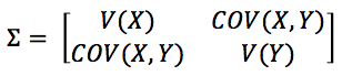
This figure from Wikipedia is also quite interesting - the numbers by each dataset are the correlation coefficients.

• Positive relationships have positive correlation coefficients (independent of the slope).
• Negative relationships have negative correlation coefficients.
• Non-linear relationships such as those in the bottom row can have correlation coefficients of zero, even though there is a clear relationship, because correlation only measures whether data points with extreme values in X also have extreme values in Y -
  • That is, correlation tests for a linear relationship.